NumPy Einsum for Scientific Computing

Introduction

In scientific computing, performing efficient linear algebra operations is essential. NumPy, a fundamental Python library for numerical computations, provides numerous tools for these operations. Among these tools, einsum (Einstein Summation) stands out as a particularly powerful function for expressing complex array operations concisely.

This tutorial will guide you through understanding what einsum is and how to effectively use it in your Python code. By the end of this lab, you will be able to perform various array operations using the einsum function and understand its advantages over traditional NumPy functions.

Understanding NumPy Einsum Basics

Einstein Summation (einsum) is a powerful NumPy function that allows you to express many array operations using a concise notation. It follows the Einstein summation convention, which is commonly used in physics and mathematics to simplify complex equations.

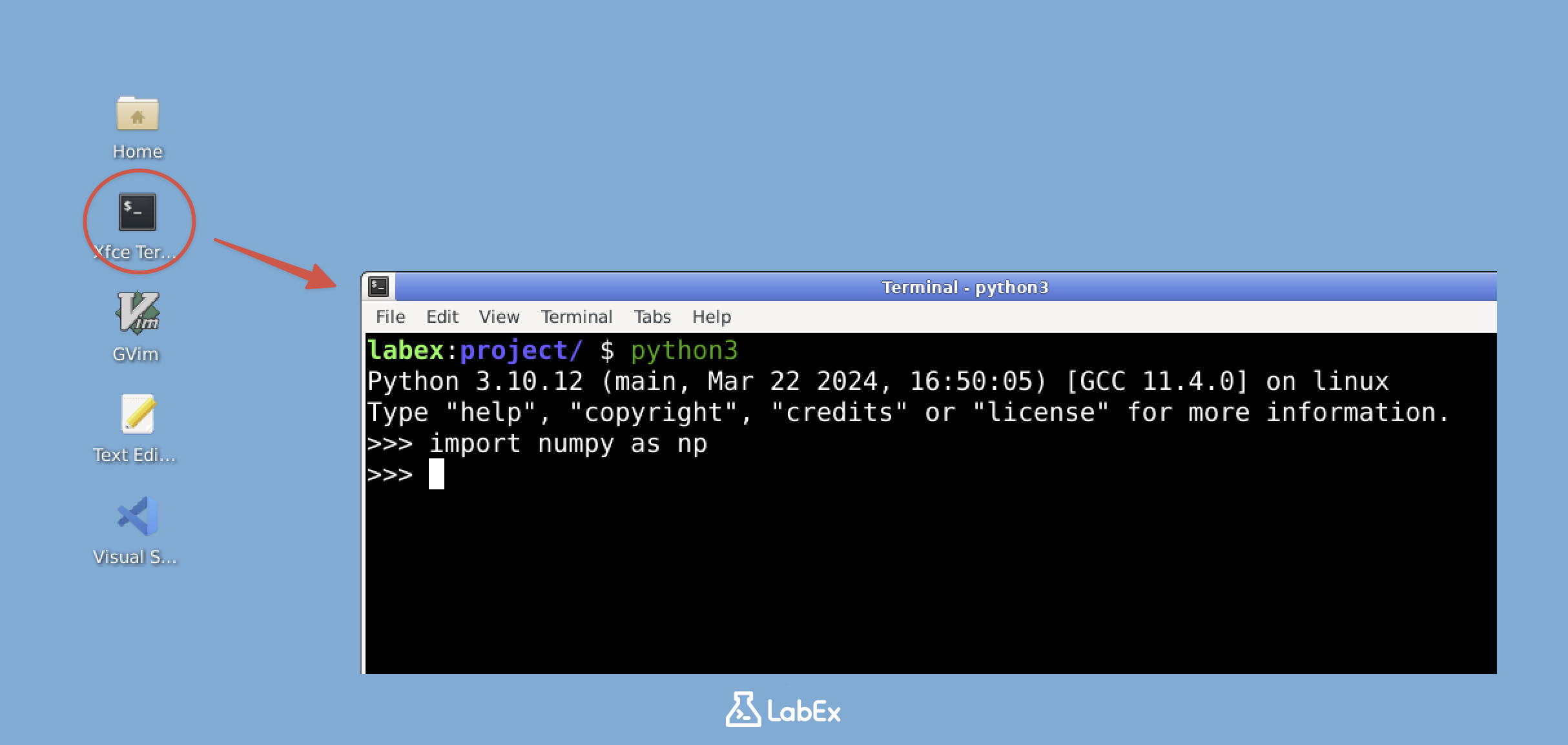
Opening the Python Shell

Let's start by opening the Python shell. Open a terminal in the Desktop and type:

python3

You should see the Python prompt (>>>), indicating that you are now in the Python interactive shell.

Importing NumPy

First, we need to import the NumPy library:

import numpy as np

What is Einsum?

The einsum function in NumPy allows you to specify array operations using a string notation that describes which indices (dimensions) of the arrays should be operated on.

The basic format of an einsum operation is:

np.einsum('notation', array1, array2, ...)

Where the notation string describes the operation to be performed.

A Simple Example: Vector Dot Product

Let's start with a simple example: calculating the dot product of two vectors. In mathematical notation, the dot product of two vectors u and v is:

\sum_i u_i \times v_i

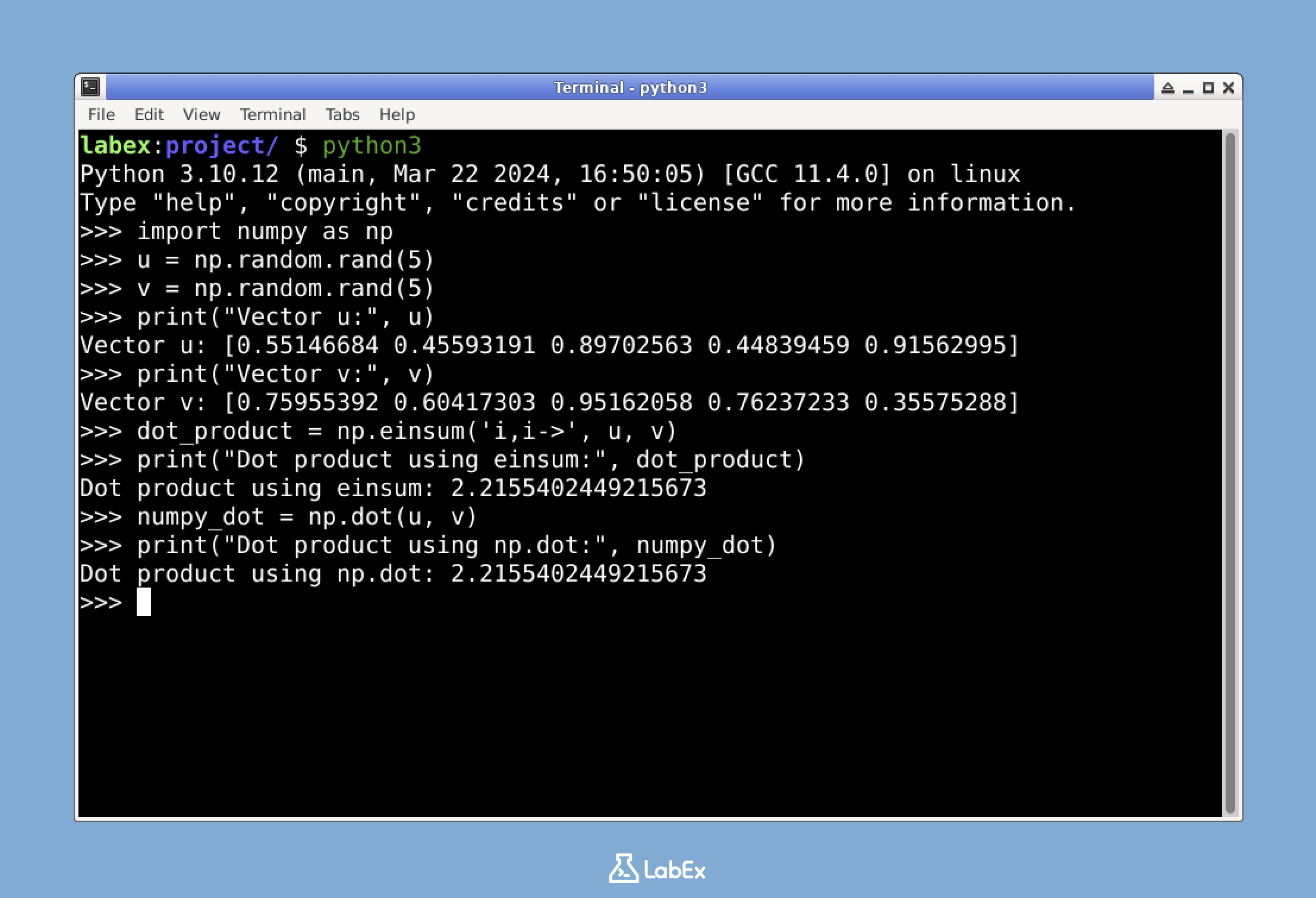
Here's how to compute it using einsum:

## Create two random vectors
u = np.random.rand(5)
v = np.random.rand(5)

## Print the vectors to see their values
print("Vector u:", u)
print("Vector v:", v)

## Calculate dot product using einsum
dot_product = np.einsum('i,i->', u, v)
print("Dot product using einsum:", dot_product)

## Verify with NumPy's dot function
numpy_dot = np.dot(u, v)
print("Dot product using np.dot:", numpy_dot)

The notation 'i,i->' means:

• i represents the index of the first array (u)
• The second i represents the index of the second array (v)
• The arrow -> followed by nothing indicates we want a scalar result (sum over all indices)

Understanding the Einsum Notation

The einsum notation follows this general pattern:

'index1,index2,...->output_indices'

• index1, index2: Labels for the dimensions of each input array
• output_indices: Labels for the dimensions in the output array
• Repeated indices across input arrays are summed over
• Indices that appear in the output are kept in the result

For example, in the notation 'ij,jk->ik':

• i, j are the dimensions of the first array
• j, k are the dimensions of the second array
• j appears in both input arrays, so we sum over this dimension
• i, k appear in the output, so these dimensions are kept

This is exactly the formula for matrix multiplication!

Common Einsum Operations

Now that we understand the basics of einsum, let's explore some common operations that we can perform using this powerful function.

Matrix Transpose

Transposing a matrix means switching its rows and columns. In mathematical notation, if A is a matrix, its transpose A^T is defined as:

A^T_{ij} = A_{ji}

Let's see how to perform matrix transposition using einsum:

## Create a random matrix
A = np.random.rand(3, 4)
print("Original matrix A:")
print(A)
print("Shape of A:", A.shape)  ## Should be (3, 4)

## Transpose using einsum
A_transpose = np.einsum('ij->ji', A)
print("\nTransposed matrix using einsum:")
print(A_transpose)
print("Shape of transposed A:", A_transpose.shape)  ## Should be (4, 3)

## Verify with NumPy's transpose function
numpy_transpose = A.T
print("\nTransposed matrix using A.T:")
print(numpy_transpose)

The notation 'ij->ji' means:

• ij represents the indices of the input matrix (i for rows, j for columns)
• ji represents the indices of the output matrix (j for rows, i for columns)
• We're essentially swapping the positions of the indices

Matrix Multiplication

Matrix multiplication is a fundamental operation in linear algebra. For two matrices A and B, their product C is defined as:

C_{ik} = \sum_j A_{ij} \times B_{jk}

Here's how to perform matrix multiplication using einsum:

## Create two random matrices
A = np.random.rand(3, 4)  ## 3x4 matrix
B = np.random.rand(4, 2)  ## 4x2 matrix

print("Matrix A shape:", A.shape)
print("Matrix B shape:", B.shape)

## Matrix multiplication using einsum
C = np.einsum('ij,jk->ik', A, B)
print("\nResult matrix C using einsum:")
print(C)
print("Shape of C:", C.shape)  ## Should be (3, 2)

## Verify with NumPy's matmul function
numpy_matmul = np.matmul(A, B)
print("\nResult matrix using np.matmul:")
print(numpy_matmul)

The notation 'ij,jk->ik' means:

• ij represents the indices of matrix A (i for rows, j for columns)
• jk represents the indices of matrix B (j for rows, k for columns)
• ik represents the indices of the output matrix C (i for rows, k for columns)
• The repeated index j is summed over (matrix multiplication)

Element-wise Multiplication

Element-wise multiplication involves multiplying corresponding elements of two arrays. For two matrices A and B with the same shape, their element-wise product C is:

C_{ij} = A_{ij} \times B_{ij}

Here's how to perform element-wise multiplication using einsum:

## Create two random matrices of the same shape
A = np.random.rand(3, 3)
B = np.random.rand(3, 3)

print("Matrix A:")
print(A)
print("\nMatrix B:")
print(B)

## Element-wise multiplication using einsum
C = np.einsum('ij,ij->ij', A, B)
print("\nElement-wise product using einsum:")
print(C)

## Verify with NumPy's multiply function
numpy_multiply = A * B
print("\nElement-wise product using A * B:")
print(numpy_multiply)

The notation 'ij,ij->ij' means:

• ij represents the indices of matrix A
• ij represents the indices of matrix B
• ij represents the indices of the output matrix C
• No indices are summed over, meaning we're just multiplying corresponding elements

Advanced Einsum Operations

Now that we're comfortable with basic einsum operations, let's explore some more advanced applications. These operations demonstrate the true power and flexibility of the einsum function.

Diagonal Extraction

Extracting the diagonal elements of a matrix is a common operation in linear algebra. For a matrix A, its diagonal elements form a vector d where:

d_i = A_{ii}

Here's how to extract the diagonal using einsum:

## Create a random square matrix
A = np.random.rand(4, 4)
print("Matrix A:")
print(A)

## Extract diagonal using einsum
diagonal = np.einsum('ii->i', A)
print("\nDiagonal elements using einsum:")
print(diagonal)

## Verify with NumPy's diagonal function
numpy_diagonal = np.diagonal(A)
print("\nDiagonal elements using np.diagonal():")
print(numpy_diagonal)

The notation 'ii->i' means:

• ii represents the repeated index for the diagonal elements of A
• i means we extract these elements into a 1D array

Matrix Trace

The trace of a matrix is the sum of its diagonal elements. For a matrix A, its trace is:

\text{trace}(A) = \sum_i A_{ii}

Here's how to calculate the trace using einsum:

## Using the same matrix A from above
trace = np.einsum('ii->', A)
print("Trace of matrix A using einsum:", trace)

## Verify with NumPy's trace function
numpy_trace = np.trace(A)
print("Trace of matrix A using np.trace():", numpy_trace)

The notation 'ii->' means:

• ii represents the repeated index for the diagonal elements
• The empty output index means we sum all diagonal elements to get a scalar

Batch Matrix Multiplication

einsum really shines when performing operations on higher-dimensional arrays. For example, batch matrix multiplication involves multiplying pairs of matrices from two batches.

If we have a batch of matrices A with shape (n, m, p) and a batch of matrices B with shape (n, p, q), batch matrix multiplication gives us a result C with shape (n, m, q):

C_{ijk} = \sum_l A_{ijl} \times B_{ilk}

Here's how to perform batch matrix multiplication using einsum:

## Create batches of matrices
n, m, p, q = 5, 3, 4, 2  ## Batch size and matrix dimensions
A = np.random.rand(n, m, p)  ## Batch of 5 matrices, each 3x4
B = np.random.rand(n, p, q)  ## Batch of 5 matrices, each 4x2

print("Shape of batch A:", A.shape)
print("Shape of batch B:", B.shape)

## Batch matrix multiplication using einsum
C = np.einsum('nmp,npq->nmq', A, B)
print("\nShape of result batch C:", C.shape)  ## Should be (5, 3, 2)

## Let's check the first matrix multiplication in the batch
print("\nFirst result matrix from batch using einsum:")
print(C[0])

## Verify with NumPy's matmul function
numpy_batch_matmul = np.matmul(A, B)
print("\nFirst result matrix from batch using np.matmul:")
print(numpy_batch_matmul[0])

The notation 'nmp,npq->nmq' means:

• nmp represents the indices of batch A (n for batch, m for rows, p for columns)
• npq represents the indices of batch B (n for batch, p for rows, q for columns)
• nmq represents the indices of the output batch C (n for batch, m for rows, q for columns)
• The repeated index p is summed over (matrix multiplication)

Why Use Einsum?

You might wonder why we should use einsum when NumPy already provides specialized functions for these operations. Here are some advantages:

1. Unified Interface: einsum provides a single function for many array operations
2. Flexibility: It can express operations that would otherwise require multiple steps
3. Readability: Once you understand the notation, the code becomes more concise
4. Performance: In many cases, einsum operations are optimized and efficient

For complex tensor operations, einsum often provides the clearest and most direct implementation.

Summary

In this lab, you have explored the powerful einsum function in NumPy, which implements Einstein summation convention for array operations. Let's recap what you have learned:

1. Basic Einsum Concepts: You learned how to use the einsum notation to express array operations, with indices representing array dimensions and repeated indices indicating summation.

2. Common Operations: You implemented several fundamental operations using einsum:

   • Vector dot product
   • Matrix transpose
   • Matrix multiplication
   • Element-wise multiplication

3. Advanced Applications: You explored more complex operations:

   • Diagonal extraction
   • Matrix trace
   • Batch matrix multiplication

The einsum function provides a unified and flexible approach to array operations in NumPy. While specialized functions like np.dot, np.matmul, and np.transpose are available for specific operations, einsum offers a consistent interface for a wide range of operations, which becomes especially valuable when working with higher-dimensional arrays.

As you continue your journey in scientific computing and data science, einsum will be a powerful tool in your arsenal for performing complex array operations with concise and readable code.