Linear Regression Fitting and Plotting

Introduction

In this project, you will learn how to perform linear regression on a set of data points and visualize the results using Matplotlib. Linear regression is a fundamental machine learning technique used to model the relationship between a dependent variable (y) and one or more independent variables (x).

🎯 Tasks

In this project, you will learn:

• How to convert the given data to a Numpy array for easier manipulation
• How to calculate the coefficients of the linear regression model, including the slope (w) and the intercept (b)
• How to plot the data points on a scatter plot and draw the linear regression line on the same plot

🏆 Achievements

After completing this project, you will be able to:

• Prepare data for linear regression analysis
• Use Numpy functions to calculate the linear regression parameters
• Create a scatter plot and overlay the linear regression line using Matplotlib
• Gain a better understanding of linear regression and its practical applications in data analysis and visualization

Skills Graph

Convert Data to NumPy Array

In this step, you will learn how to convert the given data to a NumPy array for easier manipulation.

Open the linear_regression_plot.py file.

Locate the data variable at the beginning of the linear_plot() function.

Convert the data list to a NumPy array using the np.array() function.

data = np.array(data)

Now, the data variable is a NumPy array, which will make it easier to work with in the next steps.

Calculate Linear Regression Parameters

In this step, you will learn how to calculate the values of the coefficient w and the intercept b from the data.

Continue in the linear_plot() function, extract the x and y values from the NumPy array data.

x = data[:, 0]
y = data[:, 1]

Use the np.polyfit() function to calculate the linear regression parameters w and b.

w, b = np.polyfit(x, y, 1)

Round the calculated values of w and b to two decimal places using the round() function.

w = round(w, 2)
b = round(b, 2)

Now, you have the values of the coefficient w and the intercept b ready to be used in the next step.

Plot the Linear Regression Line

In this step, you will learn how to plot the sample scatter plot and draw the fitting line on the graph based on the calculated parameters.

Continue in the linear_plot() function, create a new Matplotlib figure and axis using plt.subplots().

fig, ax = plt.subplots()

Plot the data points using the ax.scatter() function.

ax.scatter(x, y, label="Data Points")

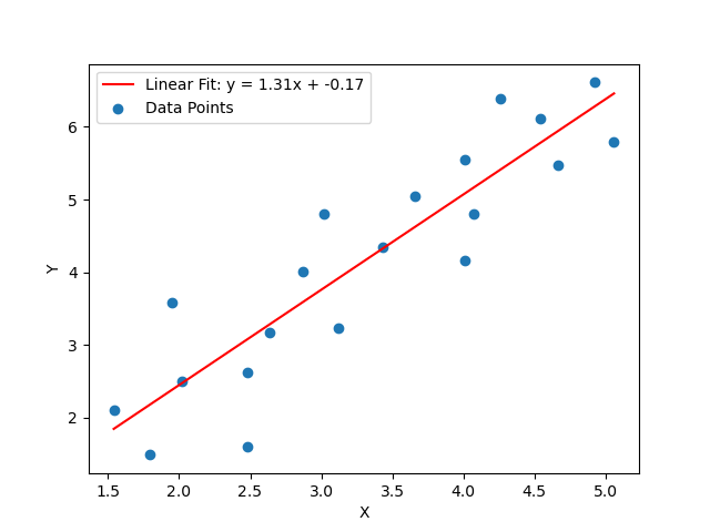
Plot the linear regression line using the ax.plot() function and the calculated values of w and b.

ax.plot(x, w * x + b, color="red", label=f"Linear Fit: y = {w}x + {b}")

Add labels and a legend to the plot.

ax.set_xlabel("X")
ax.set_ylabel("Y")
ax.legend()

Finally, return the values of w, b, and the fig object.

return w, b, fig

Now, you have completed the linear_plot() function, which performs linear regression on the given data and returns the coefficients and the Matplotlib plot object.

Run the Linear Regression Plot

In this final step, you will learn how to execute your script to see the linear regression plot in action. This part of the code will use the functions defined earlier in the linear_plot() to display the scatter plot along with the linear regression line.

The provided Python snippet will check if the script is being run as the main program and, if so, it will call the linear_plot() function and display the resulting plot.

if __name__ == "__main__":
    ## Call the linear_plot function to compute the regression parameters and generate the plot
    w, b, fig = linear_plot()
    ## Display the plot
    plt.show()

Here, if __name__ == "__main__": ensures that the linear_plot() function is called only when the script is run directly, not when imported as a module. After calling linear_plot(), which returns the slope w, intercept b, and the figure object fig, plt.show() is used to display the plot in a window. This allows you to visually inspect the fit of the regression line to the data.

Now you can press the "Run Cell" button at the top of the first line of `linear_regression_plot.py' and see the result.

With this setup, you can easily rerun the script with different data sets or adjustments to the regression calculation to see immediate visual feedback.

Summary

Congratulations! You have completed this project. You can practice more labs in LabEx to improve your skills.