
Introduction
Welcome to this hands-on lab on K-Nearest Neighbors (KNN) classification using scikit-learn! Scikit-learn is a powerful and popular Python library for machine learning. The KNN algorithm is one of the simplest yet effective classification algorithms. It classifies a new data point based on the majority class of its 'k' nearest neighbors in the feature space. In this lab, you will walk through the complete process of building a machine learning model: loading the famous Iris dataset, splitting it into training and testing sets, initializing and training a KNN classifier, and finally, using the trained model to make predictions on new, unseen data. By the end of this lab, you will have a solid understanding of the fundamental workflow for supervised learning in scikit-learn.
Load Iris dataset with datasets.load_iris()
In this step, you will begin by loading the necessary dataset. We will use the classic Iris dataset, which is conveniently included with scikit-learn. First, you need to import the datasets module from sklearn. Then, you'll call the load_iris() function to get the data.
Understanding load_iris():
- Return type: Returns a
Bunchobject (similar to a dictionary) containing:.data: Feature matrix (150 samples × 4 features: sepal length, sepal width, petal length, petal width).target: Label array (species: 0=setosa, 1=versicolor, 2=virginica).feature_names: Names of the 4 features.target_names: Names of the 3 species
- Purpose: Provides a clean, ready-to-use dataset for classification practice
We will assign these to variables X and y, respectively, which is a common convention in machine learning (X for features, y for labels).
Open the main.py file in the editor on the left and add the following code.
from sklearn import datasets

## Load the iris dataset
iris = datasets.load_iris()

## Assign features to X and labels to y
X = iris.data
y = iris.target

## You can print the shape to see the dimensions
print("Features shape:", X.shape)
print("Labels shape:", y.shape)
Now, run the script from the terminal to see the output.
python3 main.py
You should see the dimensions of the feature matrix and the label vector.
Features shape: (150, 4)
Labels shape: (150,)
This tells us we have 150 samples (flowers) and 4 features for each sample.
Split data into train and test using train_test_split from sklearn.model_selection
In this step, you will split the dataset into two parts: a training set and a testing set. This is a crucial step in machine learning to evaluate the performance of a model on unseen data.
Understanding train_test_split() parameters:
test_size=0.3: Reserves 30% of data for testing, 70% for trainingrandom_state=42: Ensures reproducible splits (same random seed each run)- Purpose: Prevents overfitting by evaluating model on unseen data
- Output: Returns four arrays: X_train, X_test, y_train, y_test
We train the model on the training set and then test its predictive power on the testing set. Scikit-learn provides a handy function called train_test_split for this purpose. You need to import it from sklearn.model_selection.
Add the following code to the end of your main.py file.
from sklearn.model_selection import train_test_split

## Split data into training and testing sets
## test_size=0.3 means 30% of the data will be used for testing
## random_state ensures reproducibility
X_train, X_test, y_train, y_test = train_test_split(X, y, test_size=0.3, random_state=42)

## Print the shapes of the new sets
print("X_train shape:", X_train.shape)
print("X_test shape:", X_test.shape)
Now, run the script again.
python3 main.py
The output will now include the shapes of your training and testing sets.
Features shape: (150, 4)
Labels shape: (150,)
X_train shape: (105, 4)
X_test shape: (45, 4)
Initialize KNeighborsClassifier with n_neighbors=3 from sklearn.neighbors
In this step, you will initialize the K-Nearest Neighbors classifier. The core idea of KNN is to predict the class of a data point by looking at the classes of its 'k' closest neighbors.
Understanding KNeighborsClassifier() parameters:
n_neighbors=3: Number of nearest neighbors to consider for prediction- Smaller values (e.g., 1-3): More sensitive to noise, can overfit
- Larger values (e.g., 5-7): Smoother decision boundaries, more robust
- Algorithm behavior: For prediction, finds k closest training points and uses majority voting
- No training phase: KNN is a "lazy learner" - it stores training data and computes during prediction
The KNeighborsClassifier is the class in scikit-learn that implements this algorithm. You need to import it from sklearn.neighbors. Let's create a classifier object and name it clf.
Add the following code to the end of your main.py file.
from sklearn.neighbors import KNeighborsClassifier

## Initialize the KNN classifier with n_neighbors=3
clf = KNeighborsClassifier(n_neighbors=3)
This code doesn't produce any output, but it creates the classifier object in memory, ready to be trained in the next step.
Fit classifier with clf.fit(X_train, y_train)
In this step, you will train, or 'fit', the classifier using your training data. For the KNN algorithm, the 'training' phase is very simple: it just involves storing the entire training dataset (X_train and y_train).
Understanding .fit() method:
- Input parameters:
X_train(feature matrix),y_train(target labels) - What it does: Stores the training data in memory for later use during prediction
- KNN specificity: Unlike other algorithms, KNN doesn't learn parameters during fit
- Purpose: Prepares the model for making predictions on new data
When a prediction is required for a new point, the algorithm finds the 'k' nearest points in this stored dataset and makes a decision. To train the model in scikit-learn, you use the .fit() method of the classifier object. The method takes the training features (X_train) and the corresponding training labels (y_train) as arguments.
Add the following line of code to the end of main.py.
## Train the classifier using the training data
clf.fit(X_train, y_train)

print("Classifier trained successfully.")
After adding the code, run the script.
python3 main.py
You will see a confirmation message that the classifier has been trained.
Features shape: (150, 4)
Labels shape: (150,)
X_train shape: (105, 4)
X_test shape: (45, 4)
Classifier trained successfully.
Predict classes with clf.predict(X_test)
In this final step, you will use the trained classifier to make predictions on the test data. Now that the model has 'learned' from the training data, we can give it the features of the test set (X_test), which it has never seen before, and ask it to predict the class for each sample.
Understanding .predict() method:
- Input parameter:
X_test(feature matrix of unseen data) - Algorithm process: For each test sample, finds k nearest neighbors in training data and uses majority voting
- Output: Array of predicted class labels (same length as input samples)
- Distance metric: Uses Euclidean distance by default to measure similarity between points
- Purpose: Evaluates model performance on new, unseen data
This is done using the .predict() method. The method takes the test features (X_test) as input and returns an array of predicted labels. We will store these predictions in a variable called predictions and print them to the console. You can also print the actual labels (y_test) to see how well the model performed.
Add the final piece of code to your main.py file.
## Make predictions on the test data
predictions = clf.predict(X_test)

print("Predictions on test data:", predictions)
print("Actual labels of test data:", y_test)
Now, run the complete script.
python3 main.py
You will see the array of predicted class labels for the test set, followed by the array of the true labels.
... (previous output) ...
Classifier trained successfully.
Predictions on test data: [1 0 2 1 1 0 1 2 1 1 2 0 0 0 0 1 2 1 1 2 0 2 0 2 2 2 2 2 0 0 0 0 1 0 0 2 1
 0 0 0 2 1 1 0 0]
Actual labels of test data: [1 0 2 1 1 0 1 2 1 1 2 0 0 0 0 1 2 1 1 2 0 2 0 2 2 2 2 2 0 0 0 0 1 0 0 2 1
 0 0 0 2 1 1 0 0]
Note: The output arrays are shown in full here. By comparing the two arrays, you can see that the predictions perfectly match the actual labels, indicating excellent model performance on this test set.
Visualize KNN Classification Results
In this bonus step, you will create visualizations to better understand your KNN classification results. Visualization helps you see how well your model performed and understand the decision boundaries created by the KNN algorithm.
Understanding data visualization in classification:
- Scatter plots: Show relationships between features and how classes are distributed
- Color coding: Different colors represent different classes (species)
- Training vs Test data: Helps understand model generalization
- Prediction accuracy: Visual comparison of predicted vs actual labels
Add the following code to the end of your main.py file to create visualizations:
import matplotlib.pyplot as plt
import numpy as np

## Create subplots for multiple visualizations
fig, axes = plt.subplots(1, 2, figsize=(15, 6))

## Plot 1: Training data with different colors for each class
scatter1 = axes[0].scatter(X_train[:, 0], X_train[:, 1], c=y_train, cmap='viridis', alpha=0.7, s=50)
axes[0].set_xlabel('Sepal Length (cm)')
axes[0].set_ylabel('Sepal Width (cm)')
axes[0].set_title('Training Data Distribution')
axes[0].legend(*scatter1.legend_elements(), title="Classes")

## Plot 2: Test data predictions vs actual labels
## Create a comparison: correct predictions vs incorrect ones
test_predictions = clf.predict(X_test)
correct_predictions = (test_predictions == y_test)

## Plot correct predictions
correct_mask = correct_predictions
scatter2_correct = axes[1].scatter(X_test[correct_mask, 0], X_test[correct_mask, 1],
                                  c=y_test[correct_mask], cmap='viridis', alpha=0.7, s=50, marker='o')

## Plot incorrect predictions with different marker
incorrect_mask = ~correct_predictions
if np.any(incorrect_mask):
    scatter2_incorrect = axes[1].scatter(X_test[incorrect_mask, 0], X_test[incorrect_mask, 1],
                                        c=test_predictions[incorrect_mask], cmap='viridis',
                                        alpha=0.7, s=80, marker='x', edgecolors='red', linewidths=2)

axes[1].set_xlabel('Sepal Length (cm)')
axes[1].set_ylabel('Sepal Width (cm)')
axes[1].set_title('Test Data: Predictions vs Actual\n(correct=●, incorrect=✕)')

## Create legend
legend_elements = [plt.Line2D([0], [0], marker='o', color='w', markerfacecolor='gray', markersize=8, label='Correct'),
                   plt.Line2D([0], [0], marker='x', color='red', markersize=8, label='Incorrect')]
axes[1].legend(handles=legend_elements)

plt.tight_layout()
plt.savefig('knn_classification_results.png', dpi=150, bbox_inches='tight')
print("Visualization saved to knn_classification_results.png")

## Additional: Show prediction accuracy
accuracy = np.mean(correct_predictions) * 100
print(f"Model Accuracy: {accuracy:.1f}%")
Run the updated script:
python3 main.py
You should see output including:
... (previous output) ...
Visualization saved to knn_classification_results.png
Model Accuracy: 100.0%
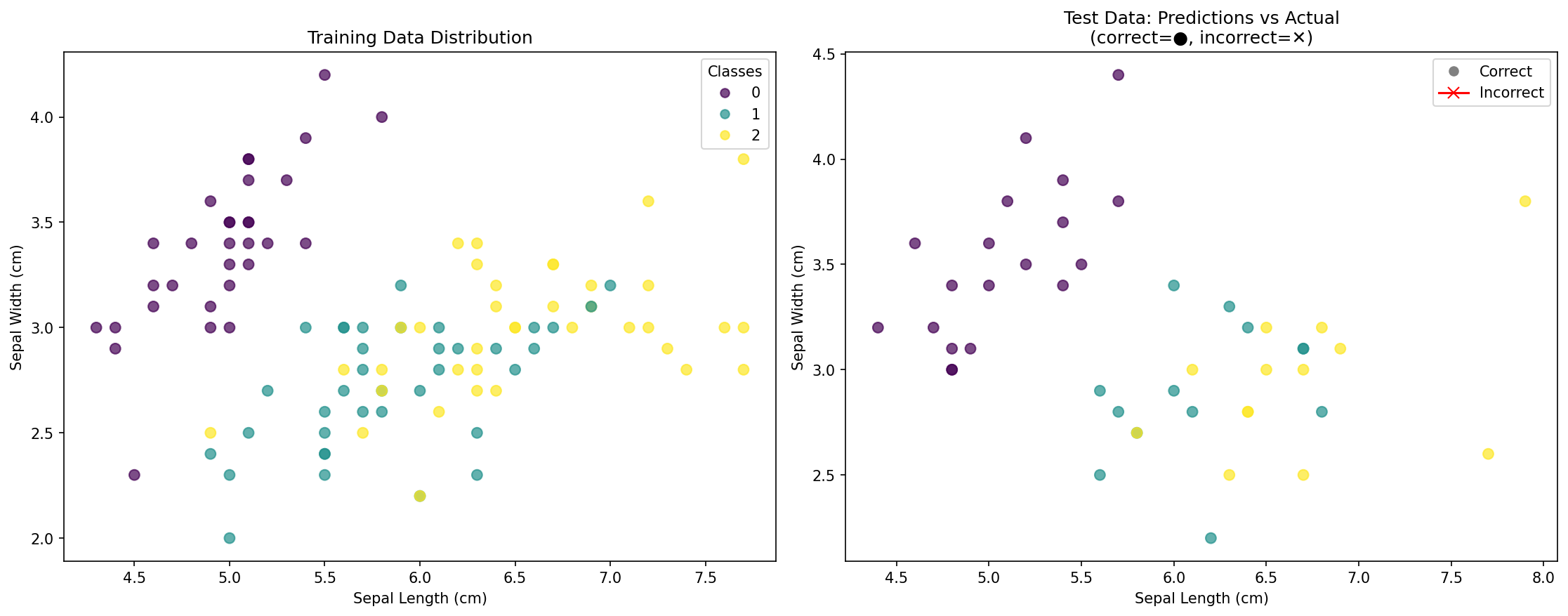
What the visualization shows:
- Left plot: Distribution of training data points, colored by their actual species
- Right plot: Test data points showing:
- Circles (●): Correctly classified points
- Crosses (✕): Incorrectly classified points (if any)
- Accuracy score: Overall percentage of correct predictions
This visualization helps you understand:
- How the classes are distributed in the feature space
- Whether your model is overfitting or generalizing well
- Which areas might be challenging for classification
- The effectiveness of your KNN model visually
Summary
Congratulations on completing this lab! You have successfully built and trained a K-Nearest Neighbors classification model using scikit-learn. You have learned the fundamental workflow of a supervised machine learning project, which includes:
- Loading a dataset using
sklearn.datasets. - Splitting the data into training and testing sets with
train_test_split. - Initializing a classifier, in this case,
KNeighborsClassifier. - Training the model on the training data using the
.fit()method. - Making predictions on new, unseen data using the
.predict()method. - Visualizing results to understand model performance and decision patterns.
This process forms the basis for many machine learning tasks. From here, you could explore how to evaluate your model's performance more formally using metrics like accuracy, precision, and recall, or experiment with different values for n_neighbors to see how it affects the outcome. You could also try visualizing decision boundaries or using different distance metrics in your KNN classifier.


