NumPy Array Creation

Introduction

Prerequisites

Before starting this course, you should have basic Python programming skills. If you haven't learned Python yet, you can start from our Python Learning Path.

Welcome to the lab on fundamental NumPy array creation techniques. Before we start coding, let's understand what NumPy is and why it's essential for scientific computing.

What is NumPy?

NumPy (short for Numerical Python) is the fundamental library for scientific computing in Python. It provides powerful data structures and functions for working with large arrays and matrices of numerical data.

Why NumPy instead of Python lists?

While Python's built-in lists are flexible and easy to use, they have limitations when working with numerical data:

• Performance: NumPy arrays are much faster for mathematical operations
• Memory efficiency: NumPy uses less memory to store the same amount of data
• Convenience: NumPy provides hundreds of built-in mathematical functions
• Functionality: NumPy supports advanced operations like matrix multiplication, Fourier transforms, etc.

In this lab, you will learn the most common methods for creating NumPy arrays. You will write and execute Python scripts to practice converting Python sequences, using built-in NumPy functions, manipulating existing arrays, and loading data from files. All coding will be done within the WebIDE.

Creating Arrays from Python Sequences

The most basic way to create a NumPy array is by converting a Python sequence, such as a list or a tuple. The numpy.array() function takes a sequence as an argument and returns a new NumPy array.

Understanding NumPy Arrays

Before we create arrays, let's understand what makes NumPy arrays special:

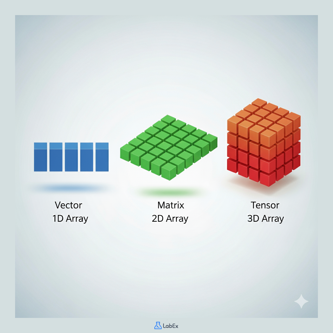
Array Dimensions

• 1D Array (Vector): A simple list of numbers, like [1, 2, 3, 4]
• 2D Array (Matrix): A table of numbers with rows and columns, like a spreadsheet
• 3D Array (Tensor): A cube of numbers, useful for images or 3D data

Key Differences from Python Lists

• Homogeneous: All elements must be the same data type (usually numbers)
• Fixed size: Once created, the size cannot be changed
• Efficient: Much faster for mathematical operations
• Rich functionality: Supports vectorized operations (operations on entire arrays at once)

Importing NumPy

In Python, we import NumPy using the standard alias np:

import numpy as np

This np alias is a widely adopted convention in the scientific Python community.

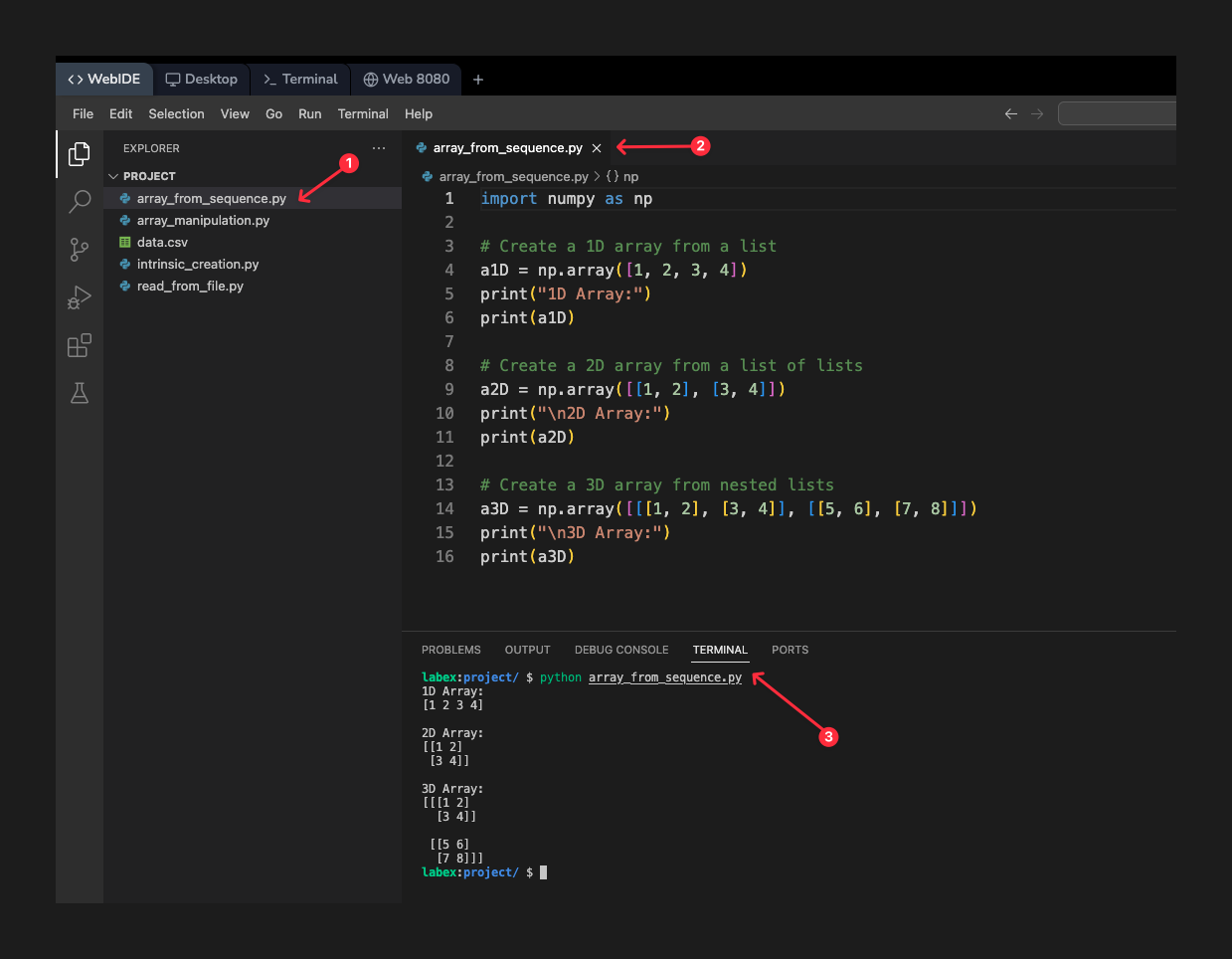
Now let's create some arrays. Open the file array_from_sequence.py from the file explorer on the left. Add the following code to it. This code will import the NumPy library and create one-dimensional (1D), two-dimensional (2D), and three-dimensional (3D) arrays from Python lists.

import numpy as np

## Create a 1D array from a list
a1D = np.array([1, 2, 3, 4])
print("1D Array:")
print(a1D)

## Create a 2D array from a list of lists
a2D = np.array([[1, 2], [3, 4]])
print("\n2D Array:")
print(a2D)

## Create a 3D array from nested lists
a3D = np.array([[[1, 2], [3, 4]], [[5, 6], [7, 8]]])
print("\n3D Array:")
print(a3D)

Suggestion: You can copy the above code into your code editor, then carefully read each line of code to understand its function. If you need further explanation, you can click the "Explain Code" button 👆. You can interact with Labby for personalized help.

After adding the code, save the file. Now, run the script from the terminal to see the output.

python array_from_sequence.py

You should see the following output, which displays the arrays you created:

1D Array:
[1 2 3 4]

2D Array:
[[1 2]
 [3 4]]

3D Array:
[[[1 2]
  [3 4]]

 [[5 6]
  [7 8]]]

Understanding Data Types (dtype)

NumPy arrays have a fixed data type for all elements, which is specified by the dtype parameter. This is different from Python lists, where each element can have a different type.

Why Data Types Matter

• Memory efficiency: Different types use different amounts of memory
• Performance: Operations are optimized for specific data types
• Precision: Controls how numbers are stored and calculated

Common Data Types

• int32 / int64: Integer numbers (32 or 64 bits)
• float32 / float64: Decimal numbers (32 or 64 bits)
• complex: Complex numbers
• bool: True/False values

You can specify the data type when creating an array using the dtype parameter, like np.array([1, 2], dtype=complex). If you don't specify a dtype, NumPy will choose an appropriate one automatically based on the input data.

Using Intrinsic Array Creation Functions

NumPy provides several built-in functions to create arrays from scratch without needing a Python sequence. These functions are optimized for specific use cases and are much faster than manually creating arrays from lists.

Why Use These Functions?

Instead of writing np.array([0, 0, 0, 0, 0]), you can simply use np.zeros(5). These functions are:

• Faster: Optimized C code under the hood
• More readable: Intent is clear from the function name
• Memory efficient: Direct memory allocation
• Convenient: No need to manually specify each element

Open the file intrinsic_creation.py and add the following code. This script demonstrates several common creation functions.

import numpy as np

## Create an array with a range of elements
## np.arange(start, stop, step) - similar to Python's range()
## Use case: Creating sequences for loops, generating indices
arr_range = np.arange(0, 10, 2)  ## [0, 2, 4, 6, 8]
print("Array from arange:")
print(arr_range)

## Create an array with a specific number of elements between two points
## np.linspace(start, stop, num_elements) - evenly spaced points
## Use case: Creating points for plotting, sampling data
arr_linspace = np.linspace(0, 10, 5)  ## 5 points from 0 to 10
print("\nArray from linspace:")
print(arr_linspace)

## Create an array filled with zeros
## np.zeros((rows, columns)) - initialize arrays for calculations
## Use case: Pre-allocating arrays before filling with computed values
arr_zeros = np.zeros((2, 3))  ## 2x3 array of zeros
print("\nArray of zeros:")
print(arr_zeros)

## Create an array filled with ones
## np.ones((rows, columns)) - initialize with ones
## Use case: Creating masks, scaling factors, or starting points for algorithms
arr_ones = np.ones((3, 2))  ## 3x2 array of ones
print("\nArray of ones:")
print(arr_ones)

## Create an identity matrix
## np.eye(size) - square matrix with 1s on diagonal, 0s elsewhere
## Use case: Linear algebra, resetting transformations, matrix multiplication
identity_matrix = np.eye(3)  ## 3x3 identity matrix
print("\nIdentity matrix:")
print(identity_matrix)

Save the file and execute it from the terminal.

python intrinsic_creation.py

The output will show the different arrays created by these functions:

Array from arange:
[0 2 4 6 8]

Array from linspace:
[ 0.   2.5  5.   7.5 10. ]

Array of zeros:
[[0. 0. 0.]
 [0. 0. 0.]]

Array of ones:
[[1. 1.]
 [1. 1.]
 [1. 1.]]

Identity matrix:
[[1. 0. 0.]
 [0. 1. 0.]
 [0. 0. 1.]]

Manipulating Existing Arrays

You can also create new arrays by modifying, combining, or splitting existing ones. This section covers two important concepts: views vs. copies and array concatenation.

Views vs. Copies: Understanding Memory Sharing

This is one of the most important concepts in NumPy that often confuses beginners.

What is a View?

A view is a different way of looking at the same data in memory. When you create a view (like through slicing), you're not creating a new array - you're just creating a new reference to the existing data.

What is a Copy?

A copy creates a completely new array in memory with its own data. Changes to a copy don't affect the original array, and vice versa.

Why This Matters

• Views are memory efficient: They don't duplicate data
• Views are fast: No copying overhead
• But views can cause unexpected side effects: Modifying a view changes the original data
• Copies are safer: Changes are isolated but use more memory

Let's also explore how to join multiple arrays into one larger array.

Open the file array_manipulation.py and add the following code:

import numpy as np

## --- Part 1: Views vs. Copies ---
a = np.arange(1, 5)
print("Original array 'a':", a)

## Create a view of the first two elements
b = a[:2]
b[0] = 99 ## Modify the view
print("Modified view 'b':", b)
print("Array 'a' after modifying the view:", a) ## 'a' is also changed

## Create a copy
c = a[:2].copy()
c[0] = 0 ## Modify the copy
print("\nModified copy 'c':", c)
print("Array 'a' after modifying the copy:", a) ## 'a' is unchanged

## --- Part 2: Joining Arrays ---
A = np.ones((2, 2))
B = np.eye(2) * 2
C = np.zeros((2, 2))
D = np.diag((-3, -4))

## Join arrays into a block matrix
block_matrix = np.block([
    [A, B],
    [C, D]
])
print("\nBlock matrix:")
print(block_matrix)

Save the file and run it from the terminal.

python array_manipulation.py

The output demonstrates how modifying a view affects the original array, while modifying a copy does not. It also shows the result of combining four smaller arrays into a single block matrix.

Original array 'a': [1 2 3 4]
Modified view 'b': [99  2]
Array 'a' after modifying the view: [99  2  3  4]

Modified copy 'c': [0 2]
Array 'a' after modifying the copy: [99  2  3  4]

Block matrix:
[[ 1.  1.  2.  0.]
 [ 1.  1.  0.  2.]
 [ 0.  0. -3.  0.]
 [ 0.  0.  0. -4.]]

Reading Arrays from a File

A common task in data analysis is to load data from a file into a NumPy array. NumPy excels at this because it can efficiently read large datasets and automatically convert them into the appropriate numerical formats.

Why NumPy for File I/O?

• Speed: Much faster than reading line-by-line with Python
• Type inference: Automatically detects appropriate data types
• Memory efficiency: Loads data directly into optimized arrays
• Convenience: Single function call instead of complex parsing

Common File Formats

• CSV files: Comma-separated values (most common)
• TSV files: Tab-separated values
• Text files: Space or custom delimiter separated
• Binary files: For very large datasets (advanced)

For simple text files like CSV (Comma-Separated Values), NumPy provides the np.loadtxt() function.

The setup script for this lab has already created a file named data.csv in your project directory. Its content is:

col1,col2,col3
1.0,2.5,3.2
4.5,5.0,6.8
7.3,8.1,9.9

Now, open the file read_from_file.py and add the following code to read this data.

Understanding np.loadtxt Parameters

The np.loadtxt() function has several important parameters:

• delimiter=',': Specifies how columns are separated (comma for CSV)
• skiprows=1: Skips the first row (usually headers)
• dtype: Optional - specifies data type (auto-detected if not provided)
• usecols: Optional - specifies which columns to read
• comments: Optional - specifies comment character to ignore lines

We use delimiter=',' to specify that columns are separated by commas and skiprows=1 to ignore the header row.

import numpy as np

## Load data from the CSV file
try:
    ## Relative paths will cause validation to fail, please use absolute paths in the lab
    data = np.loadtxt('/home/labex/project/data.csv', delimiter=',', skiprows=1)
    print("Data loaded from data.csv:")
    print(data)
except IOError:
    print("Error: data.csv not found.")

Save the file and execute it from the terminal.

python read_from_file.py

The script will read the numeric data from data.csv and print it as a NumPy array.

Data loaded from data.csv:
[[1.  2.5 3.2]
 [4.5 5.  6.8]
 [7.3 8.1 9.9]]

This method is very efficient for loading structured numerical data into arrays for further processing.

Summary

In this lab, you have learned the fundamental techniques for creating NumPy arrays. You practiced creating arrays from Python lists, using intrinsic functions like np.arange and np.zeros, manipulating existing arrays through views, copies, and joining, and loading data from a text file using np.loadtxt.

These skills are the building blocks for nearly all numerical and scientific computing tasks you will perform with Python. With a solid understanding of array creation, you are now ready to explore more advanced array manipulation and mathematical operations in NumPy.