Introduction
In this lab, you will learn the fundamentals of creating a monitoring dashboard using Grafana. Grafana is a popular open-source platform for monitoring and observability that allows you to query, visualize, alert on, and explore your metrics no matter where they are stored.
We will be working with a pre-configured environment that includes:
- Grafana: The visualization tool where you will build your dashboard.
- Prometheus: A time-series database that will serve as the data source for Grafana.
- Node Exporter: An agent that collects hardware and OS metrics from the host machine and exposes them for Prometheus to scrape.
Your goal is to build a simple dashboard from scratch that displays the live CPU usage of the lab environment.
Explore the Pre-configured Environment
In this step, you will familiarize yourself with the lab environment. The setup script has already started three Docker containers that form a basic monitoring stack.
First, let's verify that all containers are running. Open the terminal and execute the following command:
docker ps
You should see an output similar to this, listing the grafana, prometheus, and node-exporter containers. The exact container IDs will be different.
CONTAINER ID   IMAGE                           COMMAND                  CREATED          STATUS          PORTS                                       NAMES
c1a2b3c4d5e6   grafana/grafana                 "/run.sh"                15 seconds ago   Up 14 seconds   0.0.0.0:8080->3000/tcp                      grafana
f6e5d4c3b2a1   prom/prometheus                 "/bin/prometheus --c…"   20 seconds ago   Up 19 seconds   0.0.0.0:9090->9090/tcp                      prometheus
a9b8c7d6e5f4   prom/node-exporter              "/bin/node_exporter …"   25 seconds ago   Up 24 seconds   0.0.0.0:9100->9100/tcp                      node-exporter
Here's a quick breakdown of each component:
node-exporter: Collects system metrics from the virtual machine.prometheus: Scrapes and stores the metrics fromnode-exporter.grafana: Queries Prometheus and visualizes the data.
Now, let's access the Grafana user interface.
Due to LabEx VM's reverse proxy settings, switch to Desktop Interface, click the Firefox browser in the top left corner, and enter http://localhost:8080 in the address bar. You should see the Grafana login page.
Log in with the default credentials:
- Username:
admin - Password:
admin
You may be prompted to change the password. You can click Skip for this lab.

Once logged in, let's check the data source connection.
Grafana changes its left sidebar labels and icons between releases, so your screen may not match the screenshot exactly. If the sidebar is collapsed, expand it first.
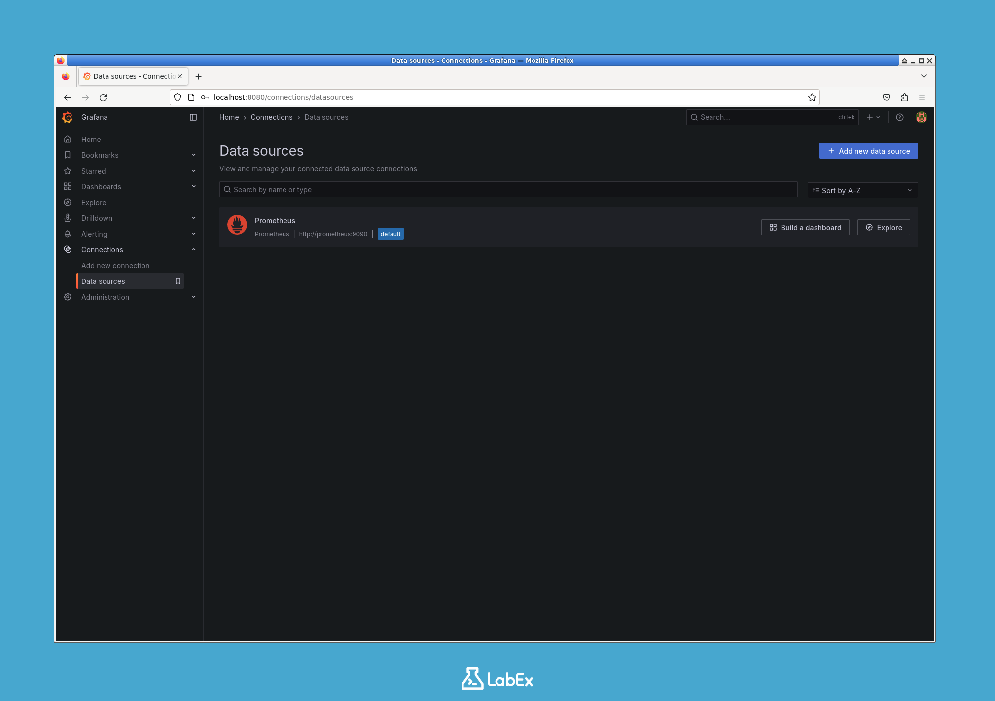
- Open the area for managing data sources. In most recent Grafana versions, use Connections and then Data sources. If you do not see Connections, use the sidebar search and open Data sources from there.
- Confirm that a pre-configured data source named
Prometheusis present. This connection was automatically set up by the initialization script, allowing Grafana to query the Prometheus container.
You are now ready to build your first dashboard.
Create New Dashboard in Grafana UI
In this step, you will create a new, empty dashboard in the Grafana interface. A dashboard is a collection of one or more panels arranged in a grid.
- In the Grafana UI, locate the left-hand sidebar.
- Create a new dashboard. The exact menu label depends on the Grafana version:
- If you see a + Create entry, open it and choose New dashboard.
- If you see Dashboards in the sidebar, open it and choose New dashboard.
- If the sidebar layout looks different, use the Grafana search box and open New dashboard from there.
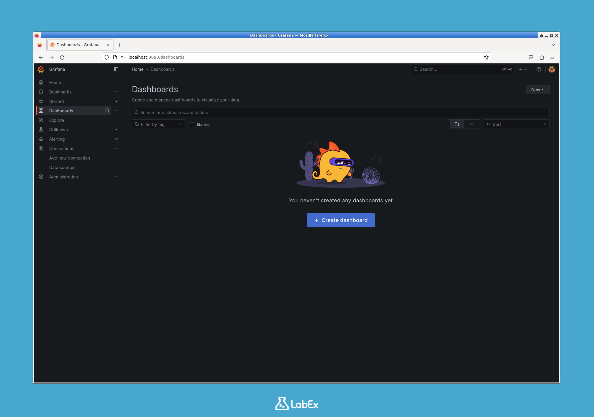
This action creates a new, empty dashboard. You are immediately prompted to add your first panel. A panel is the basic visualization building block in Grafana.
Click on the Add visualization button in the center of the screen to proceed to the panel editor.
You are now in the panel editor, where you will define your data query and customize its visualization in the next step.
Add Panel with PromQL Query for CPU Usage
In this step, you will add a panel to your dashboard and use a PromQL (Prometheus Query Language) query to fetch CPU usage data.
You should already be in the panel editor from the previous step.
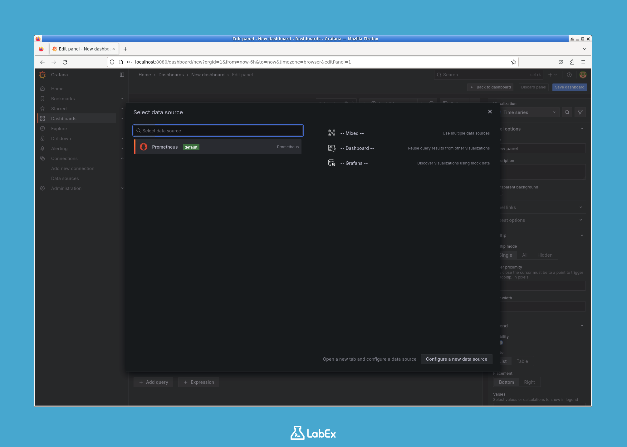
- At the bottom of the editor, you'll find the query section. The
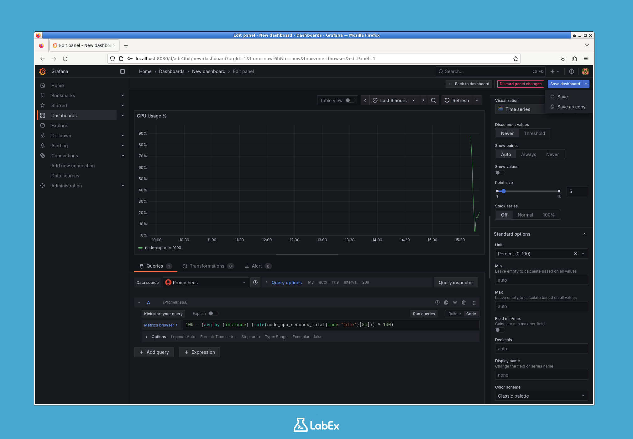
Prometheusdata source should already be selected by default. - In the Metrics browser text box, enter the following PromQL query. You can copy and paste it directly.
100 - (avg by (instance) (rate(node_cpu_seconds_total{mode="idle"}[5m])) * 100)
Let's break down this query:
node_cpu_seconds_total{mode="idle"}: This is a metric from the Node Exporter that counts the total number of seconds the CPU has been in an "idle" state.rate(...[5m]): This function calculates the per-second average rate of increase of the idle time over the last 5 minutes. The result is a value between 0 and 1, representing the fraction of time the CPU was idle.avg by (instance): This aggregates the results, which is useful if you have multiple CPUs or machines.* 100: This converts the fractional value into a percentage (e.g., 0.95 becomes 95%).100 - ...: Finally, we subtract the idle percentage from 100 to get the active CPU usage percentage.
After entering the query, a graph should automatically appear in the preview pane at the top, showing the CPU usage over time.

Your panel is now displaying data, but it can be improved with better labeling and formatting, which you will do in the next step.
Customize and Save Dashboard
In this step, you will customize the panel's appearance and save the dashboard. A well-configured panel is much easier to understand at a glance.
- On the right side of the panel editor, locate the Panel options section.
- In the Title field, enter a descriptive name for your panel, such as
CPU Usage %. You will see the title update in the preview pane. - Scroll down in the right-hand options until you find the Standard options section.
- Click on the Unit dropdown menu. It currently says "None".
- In the search box that appears, type
percentand select Percent (0-100) from the list. This will correctly format the Y-axis of your graph to display a percentage symbol.
Now that the panel is configured, apply the changes and return to the dashboard view.
- Click the Save button in the top-right corner of the screen. In some Grafana versions, this button is labeled Apply.
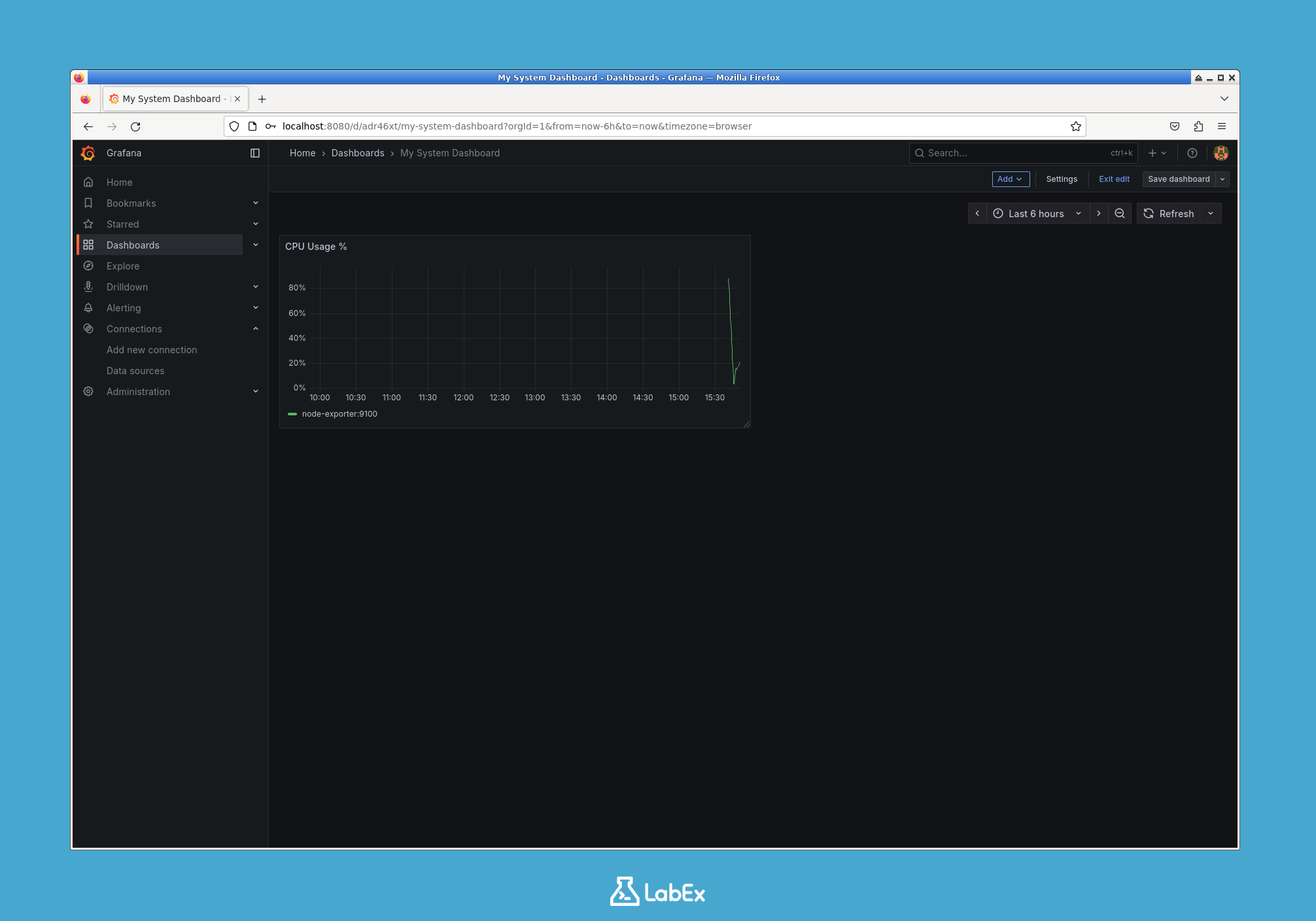
You are now back on your dashboard, which contains your newly created panel. The final step is to save the entire dashboard.
- Click the Save dashboard icon (looks like a floppy disk) in the top-right corner of the dashboard header.
- A "Save dashboard" dialog will appear. Enter the exact name
My System Dashboardso the lab can verify the saved dashboard. - Click the Save button.
Congratulations! You have successfully created and saved your first Grafana dashboard.
Summary
In this lab, you have successfully built a Grafana dashboard from scratch. You started with a pre-configured monitoring stack and performed the following key actions:
- Explored the environment consisting of Grafana, Prometheus, and Node Exporter containers.
- Navigated the Grafana UI to create a new, empty dashboard.
- Added a visualization panel and wrote a PromQL query to fetch CPU usage data from the Prometheus data source.
- Customized the panel's title and unit formatting for better readability.
- Saved the completed dashboard for future use.
You have now learned the fundamental workflow for creating visualizations in Grafana. You can build on this knowledge by adding more panels to your dashboard to monitor other system metrics like memory usage, disk I/O, or network traffic.