Creating Broken Axis Plots in Python

Introduction

Data visualization often presents challenges when dealing with outliers. These extreme values can compress the majority of your data points, making it difficult to observe important patterns or details. A broken axis plot provides an elegant solution by "breaking" the axis to show different ranges of values, allowing you to focus on both the main data distribution and the outliers simultaneously.

In this tutorial, we will learn how to create a broken axis plot using Matplotlib in Python. This technique is particularly useful when visualizing datasets with significant value disparities, enabling clearer representation of both normal data and extreme values.

VM Tips

After the VM startup is complete, click the top left corner to switch to the Notebook tab to access Jupyter Notebook for practice.

You may need to wait a few seconds for Jupyter Notebook to finish loading. Due to limitations in Jupyter Notebook, the validation of operations cannot be automated.

If you encounter any issues during this lab, feel free to ask Labby for assistance. Please provide feedback after the session so we can promptly address any problems you experienced.

Preparing the Environment and Creating Data

In this first step, we will set up our working environment by importing the necessary libraries and creating sample data for our visualization. We will focus on generating data that includes some outliers, which will demonstrate the value of using a broken axis plot.

Import Required Libraries

Let's start by importing the libraries we need for this tutorial. We will use Matplotlib for creating our visualizations and NumPy for generating and manipulating numerical data.

Create a new cell in your Jupyter Notebook and type the following code:

import matplotlib.pyplot as plt
import numpy as np

print(f"NumPy version: {np.__version__}")

When you run this cell, you should see output similar to this:

NumPy version: 2.0.0

The exact version numbers may vary depending on your environment, but this confirms the libraries are properly installed and ready to use.

Generate Sample Data with Outliers

Now, let's create a sample dataset that includes some outliers. We'll generate random numbers and then deliberately add larger values to certain positions to create our outliers.

Create a new cell and add the following code:

## Set random seed for reproducibility
np.random.seed(19680801)

## Generate 30 random points with values between 0 and 0.2
pts = np.random.rand(30) * 0.2

## Add 0.8 to two specific points to create outliers
pts[[3, 14]] += 0.8

## Display the first few data points to understand our dataset
print("First 10 data points:")
print(pts[:10])
print("\nData points containing outliers:")
print(pts[[3, 14]])

When you run this cell, you should see output similar to:

First 10 data points:
[0.01182225 0.11765474 0.07404329 0.91088185 0.10502995 0.11190702
 0.14047499 0.01060192 0.15226977 0.06145634]

Data points containing outliers:
[0.91088185 0.97360754]

In this output, you can clearly see that the values at indices 3 and 14 are much larger than the other values. These are our outliers. Most of our data points are below 0.2, but these two outliers are above 0.9, creating a significant disparity in our dataset.

This kind of data distribution is perfect for demonstrating the usefulness of a broken axis plot. In the next step, we will create the plot structure and configure it to properly display both the main data and the outliers.

Creating and Configuring the Broken Axis Plot

In this step, we will create the actual broken axis plot structure. A broken axis plot consists of multiple subplots that show different ranges of the same data. We will configure these subplots to display our main data and outliers effectively.

Create the Subplots

First, we need to create two subplots arranged vertically. The top subplot will display our outliers, while the bottom subplot will show the majority of our data points.

Create a new cell in your notebook and add the following code:

## Create two subplots stacked vertically with shared x-axis
fig, (ax1, ax2) = plt.subplots(2, 1, sharex=True, figsize=(8, 6))

## Add a main title to the figure
fig.suptitle('Broken Axis Plot Example', fontsize=16)

## Plot the same data on both axes
ax1.plot(pts, 'o-', color='blue')
ax2.plot(pts, 'o-', color='blue')

## Display the figure to see both subplots
plt.tight_layout()
plt.show()

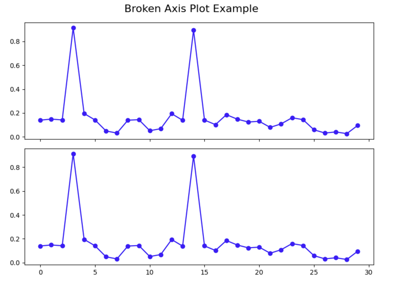
When you run this cell, you should see a figure with two subplots, both showing the same data. Notice how the outliers compress the rest of the data in both plots, making it difficult to see the details of the majority of data points. This is exactly the problem we're trying to solve with a broken axis plot.

Configure the Y-Axis Limits

Now we need to configure each subplot to focus on a specific range of y-values. The top subplot will focus on the outlier range, while the bottom subplot will focus on the main data range.

Create a new cell and add the following code:

## Create two subplots stacked vertically with shared x-axis
fig, (ax1, ax2) = plt.subplots(2, 1, sharex=True, figsize=(8, 6))

## Plot the same data on both axes
ax1.plot(pts, 'o-', color='blue')
ax2.plot(pts, 'o-', color='blue')

## Set y-axis limits for each subplot
ax1.set_ylim(0.78, 1.0)    ## Top subplot shows only the outliers
ax2.set_ylim(0, 0.22)      ## Bottom subplot shows only the main data

## Add a title to each subplot
ax1.set_title('Outlier Region')
ax2.set_title('Main Data Region')

## Display the figure with adjusted y-axis limits
plt.tight_layout()
plt.show()

When you run this cell, you should see that each subplot now focuses on a different range of y-values. The top plot shows only the outliers, and the bottom plot shows only the main data. This already improves the visualization, but to make it a proper broken axis plot, we need to add a few more configurations.

Hide the Spines and Adjust the Ticks

To create the illusion of a "broken" axis, we need to hide the connecting spines between the two subplots and adjust the tick positions.

Create a new cell and add the following code:

## Create two subplots stacked vertically with shared x-axis
fig, (ax1, ax2) = plt.subplots(2, 1, sharex=True, figsize=(8, 6))

## Plot the same data on both axes
ax1.plot(pts, 'o-', color='blue')
ax2.plot(pts, 'o-', color='blue')

## Set y-axis limits for each subplot
ax1.set_ylim(0.78, 1.0)    ## Top subplot shows only the outliers
ax2.set_ylim(0, 0.22)      ## Bottom subplot shows only the main data

## Hide the spines between ax1 and ax2
ax1.spines.bottom.set_visible(False)
ax2.spines.top.set_visible(False)

## Adjust the position of the ticks
ax1.xaxis.tick_top()          ## Move x-axis ticks to the top
ax1.tick_params(labeltop=False)  ## Hide x-axis tick labels at the top
ax2.xaxis.tick_bottom()       ## Keep x-axis ticks at the bottom

## Add labels to the plot
ax2.set_xlabel('Data Point Index')
ax2.set_ylabel('Value')
ax1.set_ylabel('Value')

plt.tight_layout()
plt.show()

When you run this cell, you should see that the plot now has hidden spines between the two subplots, creating a cleaner appearance. The x-axis ticks are now positioned correctly, with labels only at the bottom.

At this point, we have successfully created a basic broken axis plot. In the next step, we will add finishing touches to make it clear to viewers that the axis is broken.

Adding Finishing Touches to the Broken Axis Plot

In this final step, we will add finishing touches to our broken axis plot to make it clear that the y-axis is broken. We will add diagonal lines between the subplots to indicate the break, and we will improve the overall appearance of the plot with proper labels and a grid.

Add Diagonal Break Lines

To visually indicate that the axis is broken, we will add diagonal lines between the two subplots. This is a common convention that helps viewers understand that some part of the axis has been omitted.

Create a new cell and add the following code:

## Create two subplots stacked vertically with shared x-axis
fig, (ax1, ax2) = plt.subplots(2, 1, sharex=True, figsize=(8, 6))

## Plot the same data on both axes
ax1.plot(pts, 'o-', color='blue')
ax2.plot(pts, 'o-', color='blue')

## Set y-axis limits for each subplot
ax1.set_ylim(0.78, 1.0)    ## Top subplot shows only the outliers
ax2.set_ylim(0, 0.22)      ## Bottom subplot shows only the main data

## Hide the spines between ax1 and ax2
ax1.spines.bottom.set_visible(False)
ax2.spines.top.set_visible(False)

## Adjust the position of the ticks
ax1.xaxis.tick_top()          ## Move x-axis ticks to the top
ax1.tick_params(labeltop=False)  ## Hide x-axis tick labels at the top
ax2.xaxis.tick_bottom()       ## Keep x-axis ticks at the bottom

## Add diagonal break lines
d = 0.5  ## proportion of vertical to horizontal extent of the slanted line
kwargs = dict(marker=[(-1, -d), (1, d)], markersize=12,
              linestyle='none', color='k', mec='k', mew=1, clip_on=False)
ax1.plot([0, 1], [0, 0], transform=ax1.transAxes, **kwargs)
ax2.plot([0, 1], [1, 1], transform=ax2.transAxes, **kwargs)

## Add labels and a title
ax2.set_xlabel('Data Point Index')
ax2.set_ylabel('Value')
ax1.set_ylabel('Value')
fig.suptitle('Dataset with Outliers', fontsize=16)

## Add a grid to both subplots for better readability
ax1.grid(True, linestyle='--', alpha=0.7)
ax2.grid(True, linestyle='--', alpha=0.7)

plt.tight_layout()
plt.subplots_adjust(hspace=0.1)  ## Adjust the space between subplots
plt.show()

When you run this cell, you should see the complete broken axis plot with diagonal lines indicating the break in the y-axis. The plot now has a title, axis labels, and grid lines to improve readability.

Understanding the Broken Axis Plot

Let's take a moment to understand the key components of our broken axis plot:

1. Two Subplots: We created two separate subplots, each focusing on a different range of y-values.
2. Hidden Spines: We hid the connecting spines between the subplots to create a visual separation.
3. Diagonal Break Lines: We added diagonal lines to indicate that the axis is broken.
4. Y-Axis Limits: We set different y-axis limits for each subplot to focus on specific parts of the data.
5. Grid Lines: We added grid lines to improve readability and make it easier to estimate values.

This technique is especially useful when you have outliers in your data that would otherwise compress the visualization of the majority of your data points. By "breaking" the axis, you can show both the outliers and the main data distribution clearly in a single figure.

Experiment with the Plot

Now that you understand how to create a broken axis plot, you can experiment with different configurations. Try changing the y-axis limits, adding more features to the plot, or applying this technique to your own data.

For example, you can modify the previous code to include a legend, change the color scheme, or adjust the marker styles:

## Create two subplots stacked vertically with shared x-axis
fig, (ax1, ax2) = plt.subplots(2, 1, sharex=True, figsize=(8, 6))

## Plot the same data on both axes with different styles
ax1.plot(pts, 'o-', color='darkblue', label='Data Points', linewidth=2)
ax2.plot(pts, 'o-', color='darkblue', linewidth=2)

## Mark the outliers with a different color
outlier_indices = [3, 14]
ax1.plot(outlier_indices, pts[outlier_indices], 'ro', markersize=8, label='Outliers')

## Set y-axis limits for each subplot
ax1.set_ylim(0.78, 1.0)    ## Top subplot shows only the outliers
ax2.set_ylim(0, 0.22)      ## Bottom subplot shows only the main data

## Hide the spines between ax1 and ax2
ax1.spines.bottom.set_visible(False)
ax2.spines.top.set_visible(False)

## Adjust the position of the ticks
ax1.xaxis.tick_top()          ## Move x-axis ticks to the top
ax1.tick_params(labeltop=False)  ## Hide x-axis tick labels at the top
ax2.xaxis.tick_bottom()       ## Keep x-axis ticks at the bottom

## Add diagonal break lines
d = 0.5  ## proportion of vertical to horizontal extent of the slanted line
kwargs = dict(marker=[(-1, -d), (1, d)], markersize=12,
              linestyle='none', color='k', mec='k', mew=1, clip_on=False)
ax1.plot([0, 1], [0, 0], transform=ax1.transAxes, **kwargs)
ax2.plot([0, 1], [1, 1], transform=ax2.transAxes, **kwargs)

## Add labels and a title
ax2.set_xlabel('Data Point Index')
ax2.set_ylabel('Value')
ax1.set_ylabel('Value')
fig.suptitle('Dataset with Outliers - Enhanced Visualization', fontsize=16)

## Add a grid to both subplots for better readability
ax1.grid(True, linestyle='--', alpha=0.7)
ax2.grid(True, linestyle='--', alpha=0.7)

## Add a legend to the top subplot
ax1.legend(loc='upper right')

plt.tight_layout()
plt.subplots_adjust(hspace=0.1)  ## Adjust the space between subplots
plt.show()

When you run this enhanced code, you should see an improved visualization with outliers specifically marked and a legend explaining the data points.

Congratulations! You have successfully created a broken axis plot in Python using Matplotlib. This technique will help you create more effective visualizations when dealing with data that contains outliers.

Summary

In this tutorial, you learned how to create a broken axis plot using Matplotlib in Python. This visualization technique is valuable when dealing with data that contains outliers, as it allows you to display both the main data distribution and the outliers clearly in a single figure.

Here's a recap of what you accomplished:

1. Environment Setup and Data Creation: You imported the necessary libraries and created sample data containing outliers to demonstrate the concept.

2. Creating the Basic Plot Structure: You created two subplots with different y-axis limits to focus on different ranges of values and configured the appearance of the axes.

3. Enhancing the Visualization: You added diagonal break lines to indicate the broken axis, improved the plot's appearance with labels and a grid, and learned how to further customize the visualization.

The broken axis technique solves a common data visualization problem by allowing viewers to see both the overall structure and the details of a dataset simultaneously, even when outliers would normally compress the visualization of the majority of data points.

You can apply this technique to your own data analysis and visualization tasks whenever you need to represent data with significantly different value ranges in a clear and effective manner.