Scikit-learn Data Loading and Exploration

Introduction

Welcome to the world of machine learning with scikit-learn! One of the first and most crucial steps in any machine learning project is loading and understanding your data. Scikit-learn, a powerful and user-friendly library for machine learning in Python, provides several built-in datasets to help you get started.

In this lab, you will work with the famous Iris flower dataset. You will learn how to load this dataset, inspect its structure, access the feature data and target labels, and finally, create a simple visualization to get a first look at the data's distribution. This foundational knowledge is essential for any aspiring data scientist or machine learning engineer.

Load Iris dataset with datasets.load_iris()

In this step, you will learn how to load one of scikit-learn's built-in datasets. We will use the load_iris() function from the sklearn.datasets module. This function returns a "Bunch" object, which is similar to a Python dictionary and contains the dataset along with its metadata.

First, open the main.py file from the file explorer on the left side of your screen. We will write all our code in this file.

Now, add the following code to main.py to import the necessary module and load the dataset.

from sklearn import datasets

## Load the Iris dataset
iris = datasets.load_iris()

This code imports the datasets module and calls the load_iris() function, storing the resulting dataset object in a variable named iris.

To execute your script, open a terminal in the WebIDE (you can use the "Terminal" -> "New Terminal" menu) and run the following command. Your current directory is already ~/project.

python3 main.py

You will not see any output, and that's expected. We have loaded the data into the iris variable, but we haven't asked our script to print anything yet. In the next steps, we will explore the contents of this iris object.

Access data array using iris.data

In this step, you will access the core of the dataset: the feature data. The iris object we created contains an attribute called data, which holds a NumPy array of the measurements for each flower. Each row represents a sample (a flower), and each column represents a feature (a measurement).

Let's modify the main.py file to print this data array and see what it looks like.

Update your main.py file with the following code:

from sklearn import datasets

## Load the Iris dataset
iris = datasets.load_iris()

## Print the data array
print(iris.data)

Now, run the script again from your terminal:

python3 main.py

You should see a large array of numbers printed to the terminal. This is the feature data for all 150 flower samples in the dataset. Each sample has 4 features.

[[5.1 3.5 1.4 0.2]
 [4.9 3.  1.4 0.2]
 [4.7 3.2 1.3 0.2]
 ...
 [6.5 3.  5.2 2. ]
 [6.2 3.4 5.4 2.3]
 [5.9 3.  5.1 1.8]]

Access target array using iris.target

In this step, you will access the labels for each sample in the dataset. In supervised machine learning, these labels are called the "target". The iris object stores these in the target attribute. For the Iris dataset, the targets represent the species of each flower.

The species are encoded as integers: 0 for setosa, 1 for versicolor, and 2 for virginica. The iris.target attribute is a NumPy array containing the corresponding integer for each sample in iris.data.

Let's modify main.py to print the target array.

from sklearn import datasets

## Load the Iris dataset
iris = datasets.load_iris()

## Print the target array
print(iris.target)

Run the script from your terminal:

python3 main.py

The output will be an array of 0s, 1s, and 2s, representing the species for each of the 150 flowers.

[0 0 0 0 0 0 0 0 0 0 0 0 0 0 0 0 0 0 0 0 0 0 0 0 0 0 0 0 0 0 0 0 0 0 0 0 0
 0 0 0 0 0 0 0 0 0 0 0 0 0 1 1 1 1 1 1 1 1 1 1 1 1 1 1 1 1 1 1 1 1 1 1 1 1
 1 1 1 1 1 1 1 1 1 1 1 1 1 1 1 1 1 1 1 1 1 1 1 1 1 1 2 2 2 2 2 2 2 2 2 2 2
 2 2 2 2 2 2 2 2 2 2 2 2 2 2 2 2 2 2 2 2 2 2 2 2 2 2 2 2 2 2 2 2 2 2 2 2 2
 2 2]

Explore feature names with iris.feature_names

In this step, you'll learn how to find out what the columns in the iris.data array actually represent. While we know there are four features, their names are not immediately obvious from the data array itself. The iris object conveniently stores these names in the feature_names attribute.

This is very useful for understanding and interpreting your data. Let's modify main.py to print these feature names.

Update your main.py file:

from sklearn import datasets

## Load the Iris dataset
iris = datasets.load_iris()

## Print the feature names
print(iris.feature_names)

Now, run the script from your terminal:

python3 main.py

The output will be a list of strings, giving you the name for each of the four columns in iris.data.

['sepal length (cm)', 'sepal width (cm)', 'petal length (cm)', 'petal width (cm)']

Now you know that the four features correspond to the sepal length, sepal width, petal length, and petal width, all in centimeters.

Visualize data using matplotlib.pyplot.scatter(iris.data[:, 0], iris.data[:, 1])

In this final step, you will perform a simple data visualization to see the relationship between two of the features. Visualization is a key part of data exploration. We will use the matplotlib library, a popular plotting tool in Python, to create a scatter plot.

We will plot the first feature (sepal length) against the second feature (sepal width). To select these columns from our data, we use NumPy slicing:

• iris.data[:, 0] selects all rows (:) and the first column (0).
• iris.data[:, 1] selects all rows (:) and the second column (1).

Instead of displaying the plot on screen, which is not ideal for this environment, we will save it to an image file named iris_plot.png.

Update your main.py file with the following code:

from sklearn import datasets
import matplotlib.pyplot as plt

## Load the Iris dataset
iris = datasets.load_iris()

## We will plot the first two features: Sepal Length vs Sepal Width
X = iris.data[:, :2]
y = iris.target

plt.scatter(X[:, 0], X[:, 1])
plt.xlabel('Sepal Length (cm)')
plt.ylabel('Sepal Width (cm)')
plt.title('Sepal Length vs Sepal Width')

## Save the plot to a file
plt.savefig('iris_plot.png')

print("Plot saved to iris_plot.png")

Run the script from your terminal:

python3 main.py

You will see a confirmation message.

Plot saved to iris_plot.png

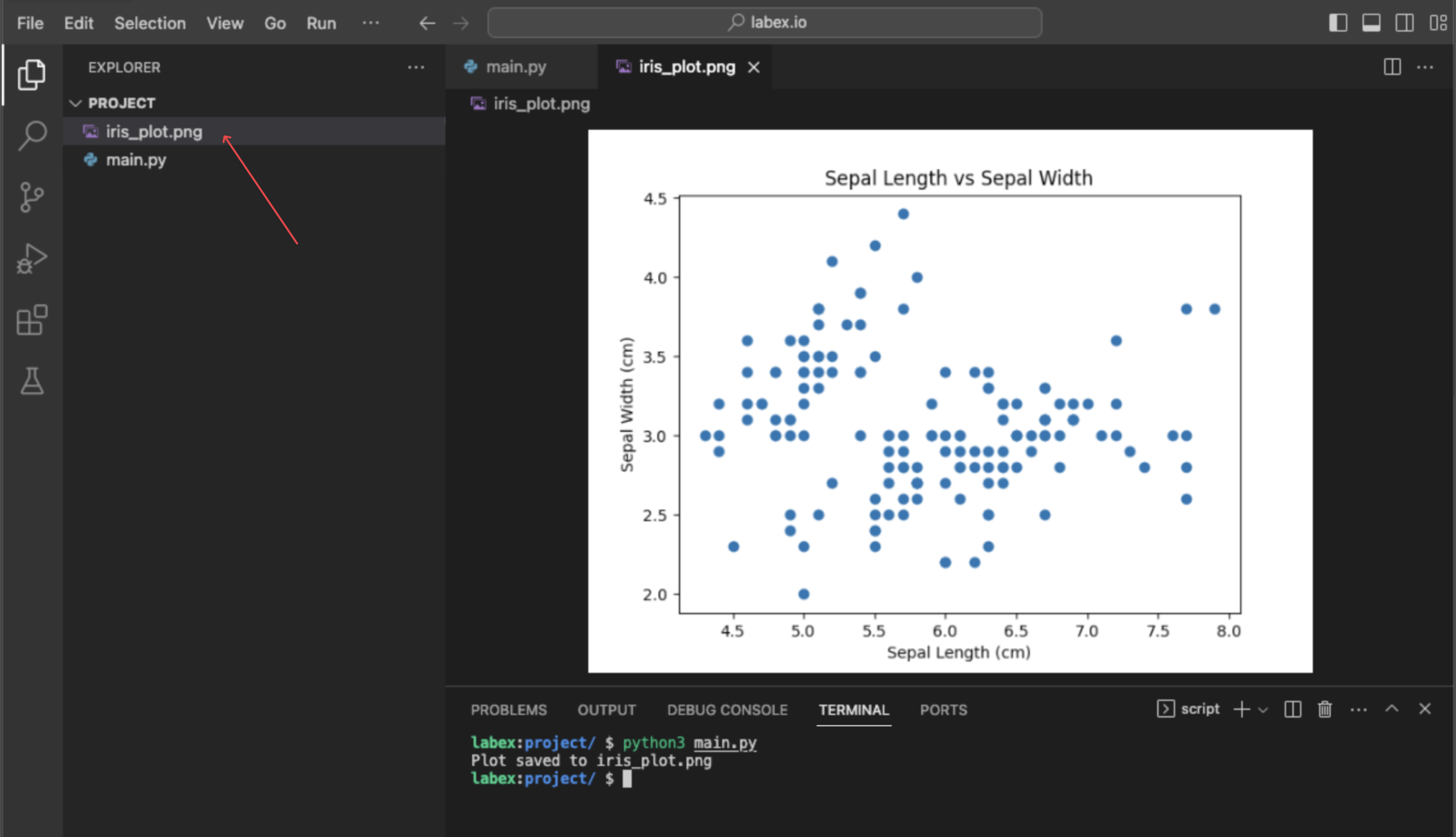
This command will not show a plot directly, but it will create a new file named iris_plot.png in your ~/project directory. You can double-click this file in the file explorer on the left to view your scatter plot.

Summary

Congratulations on completing this lab! You have successfully taken your first steps in data handling with scikit-learn.

In this lab, you learned how to:

• Load a built-in dataset using sklearn.datasets.load_iris().
• Access the feature matrix using the .data attribute.
• Access the target labels using the .target attribute.
• Understand the meaning of the features by inspecting the .feature_names attribute.
• Perform a basic data visualization by creating a scatter plot with matplotlib and saving it to a file.

These fundamental skills are the building blocks for more advanced machine learning tasks. You are now prepared to explore other datasets and begin building your own machine learning models.