Introduction
The workshop's assigned-person comparison gives page B a larger signup rate. Could random allocation alone produce different-looking groups, even if page assignment did not change anyone's outcome? A small hand exchange makes that question concrete before you generate a distribution of real randomized differences.
This independent environment already contains the correct person-building and rate-comparison functions taught in the previous lab, plus its own original data. You need those ideas, Python functions, basic NumPy arrays and introductory Matplotlib. No previous VM files or statistical inference knowledge are required. You will save 399 exploratory reassignments and their actual chart; you will not calculate a p value or choose a winner here. All records are original synthetic teaching examples. The 55-minute duration is an author estimate including reading and ordinary corrections.
Exchange People Without Changing the Group Sizes
In this step, you will calculate a six-person difference, exchange two group memberships and see why the comparison can move.
Start in WebIDE, open Terminal → New Terminal, and enter this unit's workspace:
cd /home/labex/project/signup-experiment
cat reads files without changing them. Review the worked visitor cards and the two prepared functions:
cat warmup-visitors.csv
cat outcomes.py
cat compare.py
The six cards have binary outcomes [1, 0, 0] in A and [1, 1, 0] in B. Each 1 or 0 belongs to one assigned person; repeated event rows are not additional observations. A has 1/3 signed up, B has 2/3, and B−A is about +33.33 percentage points.
Now imagine exchanging the group membership of A's second person (outcome 0) and B's first person (outcome 1). A becomes [1, 1, 0], B becomes [0, 1, 0], and the difference becomes about −33.33 percentage points. There are still three people in each group and three positive outcomes overall. You changed the allocation, not the person outcomes or the sample size.
Write the difference function. np.mean averages the binary values in a NumPy array. Multiplying B's mean minus A's mean by 100 gives percentage points. The placeholder for sample_null will be completed next; defining it does not execute it.
Shell > replaces the file. The quoted here-document <<'PY' copies the full block up to its closing PY without shell expansion. You may instead save the same content with File → Save in WebIDE.
cat > resample.py <<'PY'
import numpy as np


def difference(a, b):
    return float(100 * (np.mean(b) - np.mean(a)))


def sample_null(a, b, draws=399, seed=17):
    raise NotImplementedError("Complete this function in the next step.")
PY
The runner's contrast stage supplies the original cards and exactly the exchange just described, calls your function twice and saves both actual results:
python3 run.py contrast
The reader displays the saved artifact without rebuilding it:
python3 show_results.py contrast
Expect original_pp near +33.33 and swapped_pp near −33.33. Neither is a prediction of what would happen to a real person on another page. They show how group composition can change a comparison while the same six outcomes stay fixed.
You may edit resample.py and, later, plot.py, or add regular Python helpers beside them. Preserve the original CSVs, settings, dictionary, runner and reader. If you are in the wrong directory, use pwd and ls, then repeat the cd above. Recopy a complete function block to recover an editing mistake; setup refuses to overwrite an existing workspace.
Generate Real Reassignments
In this step, you will repeatedly reshuffle the complete visitor outcomes into groups of their original sizes and save every resulting difference.
Continue in the same WebIDE terminal at /home/labex/project/signup-experiment. The full fixed sample has 12 assigned people, six per group. Its prepared outcome function uses the complete seven-day windows. Read the actual full inputs if you want to locate the boundary and no-event people again:
cat assignments.csv
cat events.csv
Under the no-effect null assumption used for this exercise, page assignment does not change any person's binary outcome. Reassigning those fixed person outcomes between the two groups therefore shows variation expected from allocation alone. This assumption relies on the randomized-experiment design represented by these synthetic records. Shuffling an arbitrary observational website log would not create a randomized experiment.
np.concatenate([a, b]) pools the two arrays. np.random.default_rng(seed) creates a pseudorandom generator with a reproducible starting state. Its permutation method returns a shuffled copy, leaving the pooled original intact. A slice shuffled[:len(a)] takes the first A-sized section; shuffled[len(a):] takes the remaining B-sized section. Every person is used once per draw and both group sizes are preserved. Do not shuffle the repeated raw event rows.
Replace the file with both complete functions. The for loop performs the requested number of draws; append retains each calculated difference. Returning an array preserves the whole sample, rather than only its average or a favorable draw.
cat > resample.py <<'PY'
import numpy as np


def difference(a, b):
    return float(100 * (np.mean(b) - np.mean(a)))


def sample_null(a, b, draws=399, seed=17):
    pooled = np.concatenate([a, b])
    rng = np.random.default_rng(seed)
    differences = []
    for _ in range(draws):
        shuffled = rng.permutation(pooled)
        differences.append(difference(shuffled[:len(a)], shuffled[len(a):]))
    return np.array(differences)
PY
The runner calls these functions on the complete person-level sample and saves its real group counts, observed difference and 399 shuffled differences. --seed supplies the reproducible starting state; the two hyphens mark a named command option.
python3 run.py sample --seed 17
python3 show_results.py sample
The full data still has 1 of 6 signed up in A and 5 of 6 in B, an observed difference near +66.67 percentage points. null_count must be 399. The reader shows only the first eight draws as null_preview to keep the display manageable; the complete array is saved in output/sample.json.
Generate a second ordinary sample to see why a seed is not an authoritative answer:
python3 run.py sample --seed 42
python3 show_results.py sample
This replaces the saved sample with the actual seed-42 run. The sequence generally changes, while the original person outcomes, group sizes and observed comparison stay the same. Running the same seed again must reproduce the same sequence. Any nonnegative reproducible seed and equivalent independent sampling implementation are permitted; there is no required author sequence. Do not keep rerunning to find a sample that seems to favor a page. The later exact analysis uses all allocations, not whichever exploratory sample looks nicest.
Every shuffled statistic lies between −100 and +100 percentage points, though not every number in that interval is attainable. For the six-person warmup, all 20 distinct three-versus-three allocations give counts 1, 9, 9, 1 at differences −100, −100/3, +100/3, +100. The full 12-person sample has 924 allocations: their counts are 1, 36, 225, 400, 225, 36, 1 at −100, −200/3, −100/3, 0, +100/3, +200/3, +100. The next lab performs an exact computation rather than asking you to memorize these counts.
For this exploratory training task, each attainable difference's sampled frequency may differ from its exact reference frequency by at most 0.15 in absolute proportion. For example, 0.40 and 0.46 differ by 0.06. This is a deliberately broad training acceptance tolerance, not a confidence interval, a significance threshold, a business guarantee or a criterion for selecting a seed. It allows ordinary samples and independent methods without requiring identical arrays. In a legitimate all-zero example, every reassignment difference is zero; a nonzero spread is not required.
The function contract applies to the supplied binary arrays and the same bounded course variations: at least two people in each group and at most 14 overall. Checks use isolated inputs and seeds, including other group sizes, negative and zero differences and degenerate outcomes. They never replace the live sample. No sampled p value is requested or graded.
Plot the Saved Allocation Differences
In this step, you will display the actual sampled count at each difference and mark where the unchanged observed comparison lies.
Continue in the same WebIDE terminal at /home/labex/project/signup-experiment. np.unique(..., return_counts=True) returns the distinct saved differences and their occurrence counts. This is a discrete count chart: its vertical axis says how many of the 399 reassignments produced each difference. It is not an effect-confidence interval.
The plot function receives your saved result and an output path. The PNG must be at least 500 × 250 pixels to remain readable. figsize=(9, 4.5) sets the figure size in inches. DPI (dots per inch) sets the saved raster resolution: 140 pixels per inch gives about 9 × 140 by 4.5 × 140, or 1260 × 630 pixels. Matplotlib's subplots creates a figure and axes. bar draws counts, and axvline marks the observed difference without pretending it is another allocation count. A label and visible legend identify that mark. Fixed horizontal limits from −110 to +110 leave room for every possible binary-rate difference, even if an extreme value was absent from this finite sample. The vertical axis starts at zero; tight_layout leaves room for labels before savefig writes a real PNG.
cat > plot.py <<'PY'
import numpy as np
import matplotlib.pyplot as plt


def make_plot(result, destination):
    differences, counts = np.unique(result["null"], return_counts=True)
    fig, ax = plt.subplots(figsize=(9, 4.5))
    ax.bar(differences, counts, width=8, color="#6374cc", edgecolor="white")
    ax.axvline(result["difference_pp"], color="#cc5b43", linewidth=2,
               label="Observed B − A")
    ax.set_xlabel("B − A (percentage points)")
    ax.set_ylabel("Number of reassignments")
    ax.set_title("Random reassignments of the fixed visitor outcomes")
    ax.set_xlim(-110, 110)
    ax.set_ylim(0, float(max(counts)) * 1.2)
    ax.legend()
    fig.tight_layout()
    fig.savefig(destination, dpi=140)
    plt.close(fig)
PY
Read the existing saved sample and draw it with your function:
python3 run.py plot-sample
In WebIDE's file explorer, expand signup-experiment/output and open sample.png. Read the two axis labels. Most counts should cluster around a difference near zero; the red observed mark remains near +66.67 percentage points. A value absent from the sample has count zero, not an omitted person. All 399 draws and all 12 original people are still represented in the saved data.
The reference image below uses the NumPy seed-42 example just run. Another permitted sampler or seed may change the bar heights; your saved file must show your own actual draws.
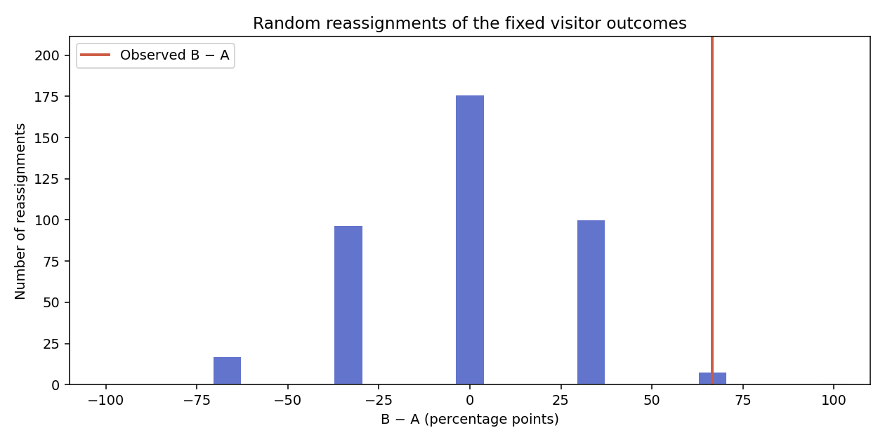
The saved PNG must be reproducible from your current plot function and saved sample. You can use readable bars, a count line or count points at the actual difference values, with a visible line or point labeled Observed at the observed difference. Keep all possible differences and the observed mark inside the displayed axes, retain the zero count baseline and label both axes. Hiding a mark, clipping the data, copying an unrelated image or plotting density while labeling it as counts does not complete this task.
If the PNG is missing, first confirm python3 show_results.py sample can read a saved sample, then rerun the plotting command. The reader itself does not generate missing files. In the next lab, you will compare an exact allocation distribution with the observed result and learn what that evidence does and does not say.
Summary
You hand-exchanged two memberships, generated 399 real fixed-size visitor reassignments and plotted their saved differences alongside the observed comparison. A reproducible seed makes a run repeatable; it does not choose an answer or a winning page. You now have the intuition needed to read the next lab's exact evidence.