Report the Evidence Without Choosing a Winner by Habit

Introduction

An exploratory reassignment plot shows how fixed visitor outcomes can produce different group comparisons. This lab takes the next step: it counts every distinct allocation in this small fixed sample, defines one precise two-sided p value and records what the evidence supports.

Correct person-building and comparison functions are already prepared in this independent environment. You need the previous labs' person-level window, percentage-point difference and fixed-size reassignment ideas, plus basic Python, NumPy and Matplotlib. You do not need files from an earlier VM or prior knowledge of p values. The records are original synthetic teaching examples, not a real business experiment; neither a large observed difference nor a small p value supplies a production guarantee. The 55-minute duration is an author estimate including reading and ordinary corrections.

Count Every Distinct Allocation

In this step, you will replace a finite randomized sample with the complete allocation distribution and calculate its explicitly defined two-sided p value.

Start in WebIDE, open Terminal → New Terminal, and enter the workspace:

cd /home/labex/project/signup-experiment

Read the source definitions and the settings before looking at the test result:

cat data-dictionary.md

cat config.json

The analysis uses a single fixed, fully followed-up sample and a single binary signup outcome per person. Its later interpretation uses the already selected alpha = 0.05. Alpha is a conventional comparison threshold for this exercise, not a 95% probability that a page works. It was not selected after searching for a favorable result. Do not change the data, the analysis instant, the threshold or the population after seeing the comparison.

Under the exercise's no-page-effect null assumption, each person's outcome would be unchanged by which page they were assigned. The represented randomized design then permits redistribution of those fixed outcomes while preserving both group sizes. This inference does not apply automatically to an arbitrary nonrandom observational log.

An exact allocation distribution includes every distinct way to place the people into the two groups. The order within a group creates no additional allocation for a mean-based statistic. Python's math.comb(n, k) counts ways to select k people from n. Here, choosing A's six people out of 12 also determines B's six.

python3 - <<'PY'
from math import comb
print("Distinct allocations:", comb(12, 6))
print("Course maximum:", comb(14, 7))
PY

The counts are 924 for this experiment and at most 3432 for any supplied course example. Exact enumeration is practical at this deliberately small size; the method is not a promise to enumerate arbitrary large production samples.

For a statistic of B−A in percentage points, this course follows SciPy's precise two-sided convention:

First find the proportion of exact allocation differences less than or equal to the observed difference. Separately find the proportion greater than or equal to it. Double the smaller of these two proportions and cap the result at 1.

Equal values belong in both respective tails. This is a defined two-sided p value; definitions are not universal. Counting abs(null) >= abs(observed) is not always equivalent for an asymmetric discrete distribution. For example, a 2-person A group with zero signups and a 5-person B group with two signups has observed +40 points. Its 21 allocations give differences −100 once, −30 ten times and +40 ten times. The defined p value is 2 * 10 / 21 = 20/21; the absolute-tail proportion would instead be 11/21. Neither grouping nor the definition may be silently changed to obtain a smaller number.

Use SciPy's prepared permutation_test interface. permutation_type="independent" redistributes observations between independent groups while preserving their sizes; it does not treat visitors as paired measurements. vectorized=False means the statistic receives ordinary one-dimensional arrays. n_resamples=np.inf requests the complete finite distribution rather than 399 random draws. alternative="two-sided" selects the convention above. No random seed is needed for this exact enumeration.

The DataFrame selection .loc[mask, "signed_up"] selects that column for matching people; .to_numpy() makes its values a one-dimensional NumPy array. The inner statistic function uses the same difference formula as the previous lab and is fully defined here, so this unit does not depend on resample.py from another VM.

result.statistic, result.pvalue and result.null_distribution are the actual computed quantities. Preserve their unrounded numeric values; .tolist() converts the array to a JSON-compatible list without removing repeated differences from different allocations.

Shell > replaces a file; the quoted here-document <<'PY' copies the complete block until the final PY without shell expansion. You may instead edit the file in WebIDE and use File → Save.

cat > inference.py <<'PY'
import numpy as np
from scipy.stats import permutation_test


def analyze(people):
    a = people.loc[people["group"] == "A", "signed_up"].to_numpy()
    b = people.loc[people["group"] == "B", "signed_up"].to_numpy()

    def statistic(x, y):
        return float(100 * (np.mean(y) - np.mean(x)))

    result = permutation_test(
        (a, b), statistic,
        permutation_type="independent",
        vectorized=False,
        n_resamples=np.inf,
        alternative="two-sided",
    )
    return {
        "difference_pp": float(result.statistic),
        "pvalue": float(result.pvalue),
        "null": result.null_distribution.tolist(),
    }
PY

The runner's distribution stage calls your analysis and saves its actual results without yet asking for an interpretation function:

python3 run.py distribution

The reader displays existing data and omits the long array only from its terminal display:

python3 show_results.py exact

Expect 12 people, group counts of 1/6 and 5/6 signed up, an observed difference near +66.67 points, null_count 924 and p near 0.08009. The full distribution remains in output/analysis.json. The interpretation field will be added in the next step.

You may edit inference.py and plot.py, or add regular Python helpers beside them. Preserve source CSVs, settings, dictionary, runner and reader. The prepared outcomes.py and compare.py implement previously taught functions; equivalent implementations are acceptable if their public DataFrame/object contracts and valid outcomes stay intact. Isolated checks cover other bounded group sizes, opposite directions, zero differences and all-zero outcomes. A fixed p value or a fixed distribution is not a reusable analysis.

For an ordinary path or filename error, use pwd and ls, repeat the starting cd, then recopy the complete block. Setup is not an editing recovery tool: it deliberately refuses to overwrite an existing workspace.

Separate Evidence from Certainty

In this step, you will add a transparent interpretation rule that can report either direction or insufficient evidence.

Continue in the same WebIDE terminal at /home/labex/project/signup-experiment. A p value describes a comparison under the chosen null assumption and allocation design. It is not the probability that the null assumption is true, not the probability that there is no page effect and not a guarantee about the next workshop.

Here, about +66.67 observed points looks large, yet the exact p value is about 0.08009. With this fixed small sample and the preselected alpha0.05, the exercise reports inconclusive evidence. That does not prove that the pages are identical. It means this particular test and sample do not provide the selected level of evidence against the null assumption.

Use these explicit output labels:

• evidence_for_b when p <= alpha and the difference is positive;
• evidence_for_a when p <= alpha and the difference is negative;
• inconclusive otherwise, including a zero difference.

Equality at the threshold belongs to the evidence branch: p == alpha satisfies <=. Do not round p before this comparison. These are bounded analysis labels, not an automatic business rollout decision. A different valid experiment may support A or neither page; no label is required to favor B.

Shell >> appends to the existing file instead of replacing it. The following complete block adds conclude below analyze; paste it once. If editing in WebIDE, add the function at the end and save. Python's and requires both conditions before a branch returns its label.

cat >> inference.py <<'PY'


def conclude(difference_pp, pvalue, alpha):
    if pvalue <= alpha and difference_pp > 0:
        return "evidence_for_b"
    if pvalue <= alpha and difference_pp < 0:
        return "evidence_for_a"
    return "inconclusive"
PY

Run the exact analysis again through the interpretation stage. This deliberately replaces the result file with a complete current analysis that also contains the label:

python3 run.py exact

python3 show_results.py exact

For this full sample, the result must say inconclusive. The observed difference, raw p value and 924 allocation differences stay the same. Do not remove people, select one date, reassign actual groups or substitute an exploratory random sample to obtain a preferred label. All required seven-day follow-up has already ended; changing a stopping rule or adding more data is outside this exercise.

Save a Readable View of the Exact Evidence

In this step, you will plot the complete saved allocation distribution and identify the observed comparison without hiding its context.

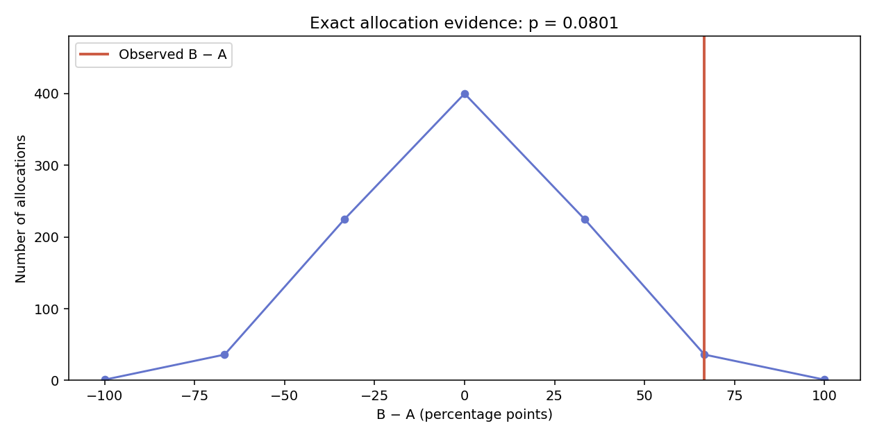
Continue in the same WebIDE terminal at /home/labex/project/signup-experiment. This chart uses the exact distribution in result["analysis"], not the exploratory sample from another unit. np.unique(..., return_counts=True) counts how many distinct allocations produce each difference; the heights must sum to 924 for the current data. Repeated values are meaningful and must not be deduplicated from the underlying distribution.

Some exact tail counts are only one allocation. Visible point markers keep these rare counts readable above the zero baseline. The connecting line helps you follow the discrete points; it does not mean that every difference between them is attainable.

The figure's horizontal coordinate is the B−A percentage-point difference and its vertical coordinate is the allocation count. The visible Observed mark locates the actual comparison. A rounded p value in a title is only a display convenience; the saved number and interpretation use the unrounded value. The full possible difference range and zero count baseline remain visible, including legitimate zeros and edge values.

Save a PNG of at least 500 × 250 pixels. As in the previous lab, a 9 × 4.5 inch figure saved at DPI 140 is about 1260 × 630 pixels; its resolution leaves room for readable axes and rare-count markers.

cat > plot.py <<'PY'
import numpy as np
import matplotlib.pyplot as plt


def make_plot(result, destination):
    analysis = result["analysis"]
    differences, counts = np.unique(analysis["null"], return_counts=True)
    fig, ax = plt.subplots(figsize=(9, 4.5))
    ax.plot(differences, counts, "o-", color="#6374cc", markersize=5)
    ax.axvline(analysis["difference_pp"], color="#cc5b43", linewidth=2,
               label="Observed B − A")
    ax.set_xlabel("B − A (percentage points)")
    ax.set_ylabel("Number of allocations")
    ax.set_title(f"Exact allocation evidence: p = {analysis['pvalue']:.4f}")
    ax.set_xlim(-110, 110)
    ax.set_ylim(0, float(max(counts)) * 1.2)
    ax.legend()
    fig.tight_layout()
    fig.savefig(destination, dpi=140)
    plt.close(fig)
PY

Generate the PNG from the actual saved analysis:

python3 run.py plot-exact

In WebIDE's file explorer, expand signup-experiment/output and open evidence.png. Look for the distribution around zero and the observed mark near +66.67. Read output/analysis.json through the reader alongside it: 12 people, the two assigned denominators, raw difference, exact p, alpha and inconclusive label form the evidence together. A chart alone is not proof of a correct analysis.

The reference below is the actual saved chart from this guided dataset and the supplied plotting code. The dots include rare allocation counts at both tails; the line only connects attainable differences. Read it alongside the saved numeric result.

You may use readable bars, a count line or count points at the actual difference values. The observed comparison needs a visible line or point labeled Observed, and both axes need meaningful labels. Keep the whole support, observed mark and zero baseline visible. The PNG must decode and reproduce from the actual saved data and current plot function; invisible strokes, off-axis marks, clipped plots and unrelated images do not pass. If the PNG is absent, first confirm the saved exact result with python3 show_results.py exact, then rerun the plotting command; the reader will not repair it.

You have analyzed one synthetic randomized-experiment sample under one stated assumption and convention. You have not measured a real business outcome, proved that the pages are identical or established that an observed effect will persist in production.

Summary

You enumerated a bounded exact allocation distribution, used a defined inclusive two-sided p value, applied a preselected threshold without rounding and saved the actual evidence chart. A large difference can remain inconclusive in a small sample; inconclusive evidence does not prove equal pages. The independent challenge now transfers this same workflow to another allocation and event history.