はじめに
この実験では、Pythonで最も人気のあるライブラリの一つである scikit-learn を使用して、機械学習モデルを構築する基礎を学びます。ここでは、価格や気温などの連続値を予測するために使用される、基本的かつ強力なアルゴリズムである「線形回帰(Linear Regression)」に焦点を当てます。
今回の目標は、カリフォルニア州の地区ごとの住宅価格の中央値を予測できるモデルを構築することです。データセットには、scikit-learn に標準で含まれているカリフォルニア住宅データセットを使用します。
この実験を通じて、以下のことを学びます:
scikit-learnからデータセットを読み込む。- 学習用とテスト用にデータを準備・分割する。
- 線形回帰モデルを作成し、学習させる。
- 学習済みモデルを使用して予測を行う。
- 結果を可視化してモデルの性能を理解する。
すべてのタスクはWebIDE内で行います。それでは始めましょう!
datasets.fetch_california_housing() でカリフォルニア住宅データセットを読み込む
このステップでは、モデル用のデータセットを読み込むことから始めます。scikit-learn には学習や練習に最適な組み込みデータセットがいくつか用意されています。今回はカリフォルニア住宅データセットを使用します。
まず、Pythonスクリプトを作成する必要があります。~/project ディレクトリには、すでに main.py というファイルが作成されています。WebIDE左側のファイルエクスプローラーで確認できます。
main.py を開き、以下のコードを追加してください。このコードは必要なライブラリ(sklearn.datasets から fetch_california_housing、および pandas)をインポートし、データセットを読み込みます。pandas を使用してデータをDataFrameに変換します。これは、データの表示や操作が容易な表形式のデータ構造です。
main.py に以下のコードを追加してください:
import pandas as pd
from sklearn.datasets import fetch_california_housing

## カリフォルニア住宅データセットを読み込む
california = fetch_california_housing()

## DataFrameを作成する
california_df = pd.DataFrame(california.data, columns=california.feature_names)
california_df['MedHouseVal'] = california.target

## DataFrameの最初の5行を表示する
print("California Housing Dataset:")
print(california_df.head())
それでは、スクリプトを実行して出力を確認しましょう。WebIDEでターミナルを開き(「Terminal」->「New Terminal」メニューを使用できます)、以下のコマンドを実行します:
python3 main.py
コンソールにデータセットの最初の5行が表示されるはずです。MedHouseVal 列がターゲット変数であり、カリフォルニアの地区ごとの住宅価格の中央値を表しています(単位は10万ドル)。
California Housing Dataset:
   MedInc  HouseAge  AveRooms  AveBedrms  Population  AveOccup  Latitude  Longitude  MedHouseVal
0  8.3252      41.0  6.984127   1.023810       322.0  2.555556     37.88    -122.23        4.526
1  8.3014      21.0  6.238137   0.971880      2401.0  2.109842     37.86    -122.22        3.585
2  7.2574      52.0  8.288136   1.073446       496.0  2.802260     37.85    -122.24        3.521
3  5.6431      52.0  5.817352   1.073059       558.0  2.547945     37.85    -122.25        3.413
4  3.8462      52.0  6.281853   1.081081       565.0  2.181467     37.85    -122.25        3.422
sklearn.model_selection の train_test_split を使用してデータを学習用とテスト用に分割する
このステップでは、学習プロセスに向けてデータを準備します。機械学習において重要なのは、モデルがこれまで見たことのないデータで評価を行うことです。そのために、データセットを「学習セット」と「テストセット」の2つに分割します。モデルは学習セットから学び、テストセットを使用してその性能を確認します。
まず、特徴量(入力変数 X)とターゲット(予測したい値 y)を分離する必要があります。今回の場合、X は MedHouseVal 以外のすべての列、y は MedHouseVal 列になります。
次に、sklearn.model_selection の train_test_split 関数を使用して分割を行います。
main.py ファイルに以下のコードを追記してください。
from sklearn.model_selection import train_test_split

## データを準備する
X = california_df.drop('MedHouseVal', axis=1)  ## 特徴量(入力変数)
y = california_df['MedHouseVal']  ## ターゲット変数(予測したい値)

## データを学習用とテスト用に分割する
## test_size=0.2: データの20%をテスト用、80%を学習用に確保
## random_state=42: 分割の再現性を確保(実行するたびに同じ結果になる)
X_train, X_test, y_train, y_test = train_test_split(X, y, test_size=0.2, random_state=42)

## 分割を確認するために新しいデータセットの形状を表示する
print("\n--- Data Split ---")
print("X_train shape:", X_train.shape)  ## 学習用特徴量
print("X_test shape:", X_test.shape)    ## テスト用特徴量
print("y_train shape:", y_train.shape)  ## 学習用ターゲット値
print("y_test shape:", y_test.shape)    ## テスト用ターゲット値
それでは、ターミナルから再度スクリプトを実行します:
python3 main.py
DataFrameの下に、新しく作成された学習用およびテスト用データセットの形状が表示されます。これでデータが正しく分割されたことが確認できました。
--- Data Split ---
X_train shape: (16512, 8)
X_test shape: (4128, 8)
y_train shape: (16512,)
y_test shape: (4128,)
sklearn.linear_model から LinearRegression モデルを初期化する
このステップでは、線形回帰モデルを作成します。scikit-learn を使えば非常に簡単です。sklearn.linear_model モジュールから LinearRegression クラスをインポートし、そのインスタンスを作成するだけです。
このインスタンスは、線形回帰アルゴリズムを含むオブジェクトです。線形回帰は、y = mx + b という式を使用してデータポイントに最も適合する直線を見つけます。ここで m は各特徴量の係数(重み)、b は切片です。ここでは、ほとんどの基本的なケースでうまく機能するデフォルトのパラメータを使用します。
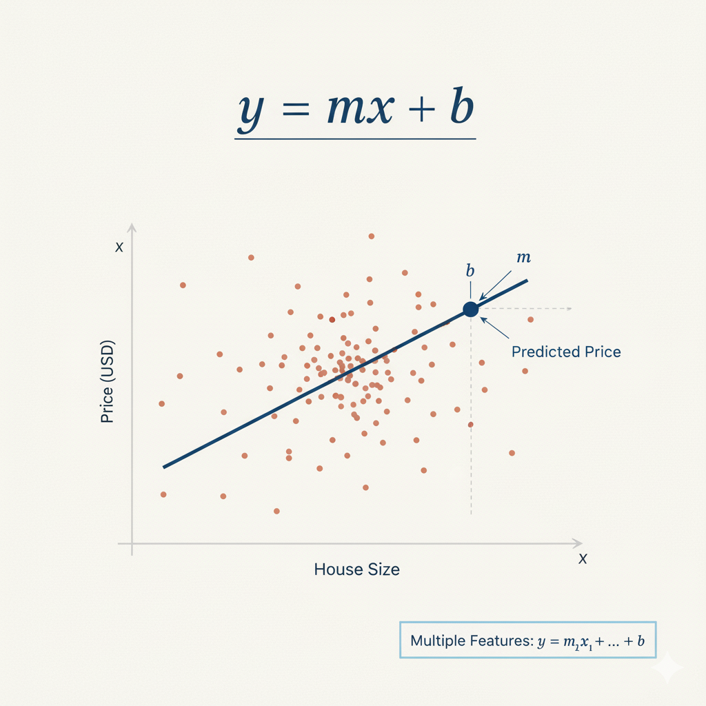 図1: 線形回帰の式 y = mx + b(mは傾き、bは切片)
main.py ファイルに以下のコードを追記してください。これにより LinearRegression クラスがインポートされ、モデルオブジェクトが作成されます。
from sklearn.linear_model import LinearRegression

## 線形回帰モデルを初期化する
model = LinearRegression()

## モデルが作成されたことを確認するために表示する
print("\n--- Model Initialized ---")
print(model)
ターミナルから main.py スクリプトを再度実行します:
python3 main.py
出力に LinearRegression オブジェクトを示す行が含まれるようになります。これでモデルが正常に初期化されたことが確認できました。
--- Model Initialized ---
LinearRegression()
model.fit(X_train, y_train) でモデルを学習させる
このステップでは、モデルを学習させます。このプロセスは、モデルをデータに「適合(fit)」させるとも呼ばれます。学習中、モデルは特徴量(X_train)とターゲット変数(y_train)の間の関係を学習します。線形回帰の場合、これはターゲットを最もよく予測できるように、各特徴量の最適な係数を見つけることを意味します。
モデルオブジェクトの fit() メソッドを使用し、学習データを引数として渡します。
main.py ファイルに以下のコードを追記してください。
## 学習データでモデルを適合(学習)させる
## fit()メソッドは、特徴量(X_train)とターゲット(y_train)の関係を学習する
## 最小二乗法を用いて、各特徴量の最適な係数と切片を計算する
model.fit(X_train, y_train)

## 学習後、モデルは係数と切片を学習している
## 切片は、すべての特徴量がゼロのときの予測値を表す
print("\n--- Model Trained ---")
print("Intercept:", model.intercept_)
それでは、ターミナルからスクリプトを実行します:
python3 main.py
スクリプトの実行後、出力に線形回帰モデルの切片を示す新しいセクションが表示されます。切片は、すべての特徴量がゼロのときの予測値です。ここに数値が表示されることで、モデルがデータに対して正常に学習されたことが確認できます。
--- Model Trained ---
Intercept: -37.023277706064185
model.predict(X_test) でテストデータに対して予測を行う
最後のステップでは、学習済みモデルを使用して予測を行います。これは予測モデルを構築する究極の目的です。学習中にモデルが見ていないテストデータ(X_test)を使用して、その性能を評価します。
学習済みモデルオブジェクトの predict() メソッドを使用し、テスト特徴量(X_test)を引数として渡します。このメソッドは、ターゲット変数の予測値の配列を返します。
main.py ファイルに以下のコードを追記してください。
## テストデータに対して予測を行う
## predict()メソッドは、学習した係数と切片を使用して予測を計算する
## 式: prediction = intercept + (coeff1 * feature1) + (coeff2 * feature2) + ...
predictions = model.predict(X_test)

## 最初の5つの予測を表示する(単位は10万ドル)
print("\n--- Predictions ---")
print(predictions[:5])
それでは、ターミナルからスクリプトを最後にもう一度実行します:
python3 main.py
出力に、テストセットに対する最初の5つの住宅価格の予測値が含まれるようになります。これらの値は、X_test の特徴量に基づいてモデルが予測した住宅価格の中央値です。これらの予測値を y_test の実際の値と比較することで、モデルの精度を概念的に評価できます。
--- Predictions ---
[0.71912284 1.76401657 2.70965883 2.83892593 2.60465725]
おめでとうございます!scikit-learn を使用して線形回帰モデルの構築、学習、および予測を成功させました。
matplotlib.pyplot.scatter() を使用してモデルの予測を可視化する
この最後のステップでは、モデルの性能をより深く理解するために可視化を行います。可視化は、生の数値だけでは明らかにならないパターンや関係性を見つけるために、機械学習において非常に重要です。
実際の住宅価格(y_test)とモデルの予測値を比較する散布図を作成します。このタイプのプロットは「予測値 vs 実測値」散布図と呼ばれます。もしモデルが完璧であれば、すべての点は予測値と実測値が等しい対角線(45度の線)上に並びます。
matplotlib を使用してこの可視化を作成し、画像ファイルとして保存します。
main.py ファイルに以下のコードを追記してください:
import matplotlib.pyplot as plt

## 実測値と予測値を比較する散布図を作成する
plt.figure(figsize=(10, 6))
plt.scatter(y_test, predictions, alpha=0.5, color='blue', edgecolors='black')

## 完璧な予測を示す対角線を追加する(予測値 = 実測値)
plt.plot([y_test.min(), y_test.max()], [y_test.min(), y_test.max()],
         'r--', linewidth=2, label='Perfect Prediction')

## ラベルとタイトルを追加する
plt.xlabel('Actual House Prices ($100,000)')
plt.ylabel('Predicted House Prices ($100,000)')
plt.title('Linear Regression: Actual vs Predicted House Prices')
plt.legend()
plt.grid(True, alpha=0.3)

## プロットをファイルに保存する
plt.savefig('housing_predictions.png', dpi=300, bbox_inches='tight')
plt.close()

print("\n--- Visualization Complete ---")
print("Plot saved to housing_predictions.png")
それでは、ターミナルからスクリプトを実行します:
python3 main.py
プロットが保存されたことを示す確認メッセージが表示されます。
--- Visualization Complete ---
Plot saved to housing_predictions.png
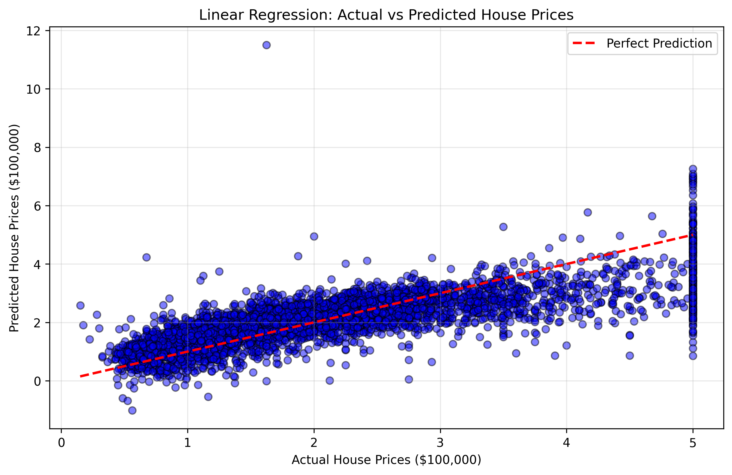 図2: 実際の住宅価格と予測価格を示す散布図。赤い対角線に近い点ほど、予測精度が高いことを示します。
この可視化により、以下のことが理解できます:
- 対角線に近い点: モデルが正確に予測できた良好なケース
- 対角線から離れた点: モデルが大きな誤差を出した不正確なケース
- 全体的なパターン: モデルが特定の価格帯で過大評価または過小評価する傾向があるかどうか
ファイルエクスプローラーで housing_predictions.png ファイルをダブルクリックすると、可視化結果を確認できます。
おめでとうございます!scikit-learn を使用して線形回帰モデルの構築、学習、テスト、および可視化を完了しました。
まとめ
この実験では、scikit-learn を使用して基本的な機械学習モデルを構築する一連のワークフローを完了しました。
まず、カリフォルニア住宅データセットを読み込み、pandas を使用して準備しました。次に、データを学習用とテスト用に分割することの重要性を学び、train_test_split を使用して分割を実行しました。
続いて、LinearRegression モデルを初期化し、fit() メソッドを使用して学習データで学習させ、predict() メソッドを使用して未知のテストデータに対して予測を行い、最後に結果を可視化してモデルの性能を評価しました。
この実験は scikit-learn の確かな基礎を提供します。ここから、以下のようなより高度なトピックを探求することができます:
- モデル評価: 平均二乗誤差(MSE)や決定係数(R-squared)などの指標を計算してモデルの精度を測定する
- データ可視化: 残差プロット、特徴量の重要度チャート、相関行列などのより高度なプロットを作成する
- 特徴量スケーリング: パフォーマンス向上のために特徴量を標準化または正規化する
- 正則化: 過学習を防ぐためにリッジ回帰やラッソ回帰を使用する
- 交差検証: k-分割交差検証を使用して、より堅牢な評価を行う
- 他のアルゴリズム: ランダムフォレスト、サポートベクターマシン、ニューラルネットワークなどを試す