NumPy の reshape: np.reshape() を使った Python 配列の変形

はじめに

NumPy ライブラリの reshape() 関数を使用すると、配列のデータを変更することなく、配列の形状を変更することができます。この強力な関数は、特定のニーズに基づいて配列要素を異なる次元に再構成するのに役立ちます。1 次元配列を行列に変換する必要がある場合でも、データ処理用の多次元配列を作成する場合でも、reshape() 関数は柔軟な解決策を提供します。

この実験では、reshape() 関数の実用的なアプリケーションを探索し、その構文を理解し、さまざまなパラメータで効果的に使用する方法を学びます。

NumPy の始め方と配列の作成

配列の形状を変更する前に、NumPy 配列とは何か、そしてそれを作成する方法を理解する必要があります。NumPy (Numerical Python) は、大規模な多次元配列や行列をサポートし、これらの配列に対して操作を行うための数学関数のコレクションを提供する強力なライブラリです。

WebIDE で新しい Python ファイルを作成して始めましょう。左側のサイドバーにある「Explorer」アイコンをクリックし、次に「New File」ボタンをクリックします。ファイル名を numpy_reshape.py とします。

New File

では、NumPy ライブラリをインポートし、基本的な配列を作成しましょう。

import numpy as np

## Create a simple 1D array using np.arange() which generates a sequence of numbers
original_array = np.arange(12)
print("Original 1D array:")
print(original_array)
print("Shape of the original array:", original_array.shape)
print("Dimensions of the original array:", original_array.ndim)

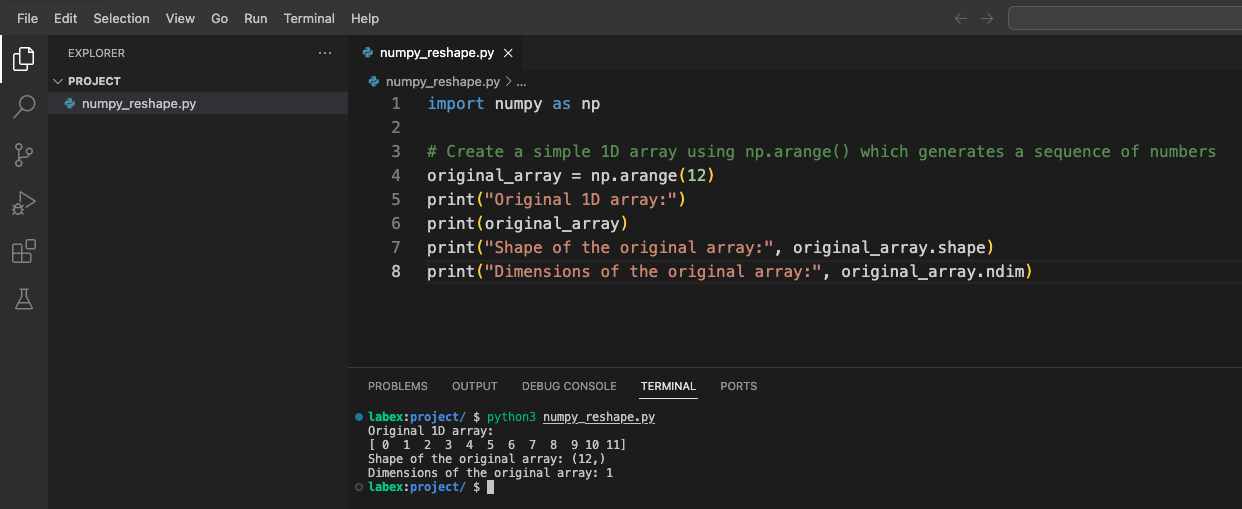
WebIDE のターミナルを開き、スクリプトを実行します。

python3 numpy_reshape.py

次のような出力が表示されるはずです。

Original 1D array:
[ 0  1  2  3  4  5  6  7  8  9 10 11]
Shape of the original array: (12,)
Dimensions of the original array: 1

ここで何が起こっているかを理解しましょう。

np.arange(12) は、0 から 11 までの値を持つ 1 次元配列を作成します。
array.shape は、配列の次元を教えてくれます（1 次元に 12 個の要素）。
array.ndim は、次元の数を教えてくれます（この場合は 1）。

基本的な形状変更 - 1 次元配列を 2 次元配列に変換する

これで NumPy 配列の基本を理解したので、reshape() 関数を探索してみましょう。この関数を使うと、配列のデータを変更することなく、配列の形状を変更することができます。

numpy_reshape.py ファイルを開き、次のコードを追加します。

import numpy as np

## Create a simple 1D array
original_array = np.arange(12)
print("Original 1D array:")
print(original_array)
print("Shape of the original array:", original_array.shape)
print("Dimensions of the original array:", original_array.ndim)
print("-" * 50)  ## Separator line

## Reshape the array to a 2D array with 3 rows and 4 columns
reshaped_3x4 = np.reshape(original_array, (3, 4))
print("Reshaped array (3x4):")
print(reshaped_3x4)
print("Shape of the reshaped array:", reshaped_3x4.shape)
print("Dimensions of the reshaped array:", reshaped_3x4.ndim)
print("-" * 50)  ## Separator line

## Reshape the array to a 2D array with 4 rows and 3 columns
reshaped_4x3 = np.reshape(original_array, (4, 3))
print("Reshaped array (4x3):")
print(reshaped_4x3)
print("Shape of the reshaped array:", reshaped_4x3.shape)
print("Dimensions of the reshaped array:", reshaped_4x3.ndim)

ターミナルでスクリプトを実行します。

python3 numpy_reshape.py

元の配列が異なる 2 次元構造に形状変更された様子を示す出力が表示されるはずです。

何が起こっているかを理解しましょう。

まず、12 個の要素を持つ 1 次元配列を作成しました。
それを 3×4 の行列（3 行、4 列）に形状変更しました。
次に、それを 4×3 の行列（4 行、3 列）に形状変更しました。

どちらの場合も、要素の総数は同じ（12）ですが、配置が変わります。reshape() 関数では、新しい形状が元の配列のサイズと互換性がある必要があります。つまり、新しい形状の次元の積は、元の配列の要素の総数と等しくなければなりません。

高度な形状変更 - 3 次元配列の作成

では、3 次元配列を作成することで、より高度な形状変更に移りましょう。3 次元配列は基本的に 2 次元配列の配列であり、ボリューム、画像の時系列、またはその他の複雑なデータ構造を表すのに役立ちます。

numpy_reshape.py ファイルに次のコードを追加します。

import numpy as np

## Create a simple 1D array
original_array = np.arange(24)
print("Original 1D array:")
print(original_array)
print("Shape of the original array:", original_array.shape)
print("-" * 50)  ## Separator line

## Reshape into a 3D array with dimensions 2x3x4
## This creates 2 blocks, each with 3 rows and 4 columns
reshaped_3d = np.reshape(original_array, (2, 3, 4))
print("Reshaped 3D array (2x3x4):")
print(reshaped_3d)
print("Shape of the 3D array:", reshaped_3d.shape)
print("Dimensions of the 3D array:", reshaped_3d.ndim)
print("-" * 50)  ## Separator line

## Accessing elements in a 3D array
print("First block of the 3D array:")
print(reshaped_3d[0])
print("\nSecond block of the 3D array:")
print(reshaped_3d[1])
print("\nElement at position [1,2,3] (second block, third row, fourth column):")
print(reshaped_3d[1, 2, 3])

再度スクリプトを実行します。

python3 numpy_reshape.py

出力では、24 個の要素を持つ 1 次元配列がどのように 3 次元構造に変換されるかが示されます。この構造は、それぞれが 3×4 の行列を含む 2 つの「ブロック」として視覚化することができます。

3 次元配列の理解：

最初の次元 (2) は、「ブロック」または「レイヤー」の数を表します。
2 番目の次元 (3) は、各ブロック内の行数を表します。
3 番目の次元 (4) は、各行内の列数を表します。

この構造は、画像処理（各「ブロック」が色チャネルである場合）、時系列データ（各「ブロック」が時点である場合）、または複数の行列を必要とするその他のシナリオで特に有用です。

Reshape におけるオーダーパラメータの理解

配列の形状を変更する際、NumPy は order という追加のパラメータを提供しています。このパラメータは、元の配列から要素を読み取り、形状変更後の配列に配置する方法を制御します。主な順序規則には 2 つあります。

C スタイルの順序（行優先）：NumPy のデフォルトで、最後の軸インデックスが最も速く変化します。
Fortran スタイルの順序（列優先）：最初の軸インデックスが最も速く変化します。

これらの順序付け方法を、numpy_reshape.py ファイルに次のコードを追加して調べてみましょう。

import numpy as np

## Create a 1D array
original_array = np.arange(12)
print("Original 1D array:")
print(original_array)
print("-" * 50)  ## Separator line

## Reshape using C-style ordering (default)
c_style = np.reshape(original_array, (3, 4), order='C')
print("Reshaped array with C-style ordering (row-major):")
print(c_style)
print("-" * 50)  ## Separator line

## Reshape using Fortran-style ordering
f_style = np.reshape(original_array, (3, 4), order='F')
print("Reshaped array with Fortran-style ordering (column-major):")
print(f_style)
print("-" * 50)  ## Separator line

## Alternative syntax using the array's reshape method
array_method = original_array.reshape(3, 4)
print("Using the array's reshape method:")
print(array_method)
print("-" * 50)  ## Separator line

## Using -1 as a dimension (automatic calculation)
auto_dim = original_array.reshape(3, -1)  ## NumPy will figure out that -1 should be 4
print("Using automatic dimension calculation with -1:")
print(auto_dim)
print("Shape:", auto_dim.shape)

違いを確認するためにスクリプトを実行します。

python3 numpy_reshape.py

理解すべき要点は次の通りです。

C スタイルの順序（行優先）：要素は行ごとに配置されます。これは NumPy のデフォルトです。
Fortran スタイルの順序（列優先）：要素は列ごとに配置されます。
配列メソッドの構文：np.reshape(array, shape) の代わりに、array.reshape(shape) を使用することができます。
自動次元計算：次元の 1 つに -1 を使用すると、NumPy は配列のサイズに基づいてその次元を自動的に計算します。

順序パラメータは、以下の場合に特に重要です。

非常に大きな配列を扱い、メモリレイアウトがパフォーマンスに影響する場合
異なるデフォルトの順序を使用する他のライブラリや言語とインターフェースする場合
特定のアルゴリズムとの互換性を確保する必要がある場合

まとめ

この実験では、NumPy の汎用的な reshape() 関数を探索しました。この関数を使用すると、基になるデータを変更することなく、配列データを異なる次元に再構成することができます。以下に学んだ内容をまとめます。

基本的な形状変更：一次元配列を、異なる行と列の構成を持つ二次元行列に変換する方法。
高度な形状変更：より複雑なデータ構造のための三次元配列を作成する方法。これは、ボリューム、画像の時系列、またはその他の多次元データを表すのに役立ちます。
順序パラメータ：C スタイル（行優先）と Fortran スタイル（列優先）の順序の違いを理解し、それらが形状変更後の配列内の要素の配置にどのように影響するかを学びました。
代替構文：np.reshape() 関数と配列の .reshape() メソッドの両方を使用して同じ結果を得る方法。
自動次元計算：-1 をプレースホルダーとして使用し、NumPy に適切な次元を自動的に計算させる方法。

reshape() 関数は、NumPy を使用したデータ操作における基本的なツールであり、データサイエンス、機械学習、および科学計算のさまざまなアプリケーションにおいて、データを効率的に再構成することができます。データを適切に形状変更する方法を理解することは、モデルへの入力を準備したり、多次元データを視覚化したり、配列に対して複雑な数学的演算を実行したりするために不可欠です。

NumPy の reshape() 関数

はじめに

NumPy の始め方と配列の作成

基本的な形状変更 - 1 次元配列を 2 次元配列に変換する

高度な形状変更 - 3 次元配列の作成

Reshape におけるオーダーパラメータの理解

まとめ