简介
在本实验中,你将学习使用最流行的 Python 库之一 scikit-learn 构建机器学习模型的基础知识。我们将重点介绍线性回归(Linear Regression),这是一种基础但功能强大的算法,用于预测连续值,例如价格或温度。
我们的目标是构建一个能够预测加利福尼亚州各地区房价中位数的模型。我们将使用 scikit-learn 中内置的加利福尼亚州住房数据集。
通过本实验,你将学会:
- 从
scikit-learn加载数据集。 - 准备并拆分数据用于训练和测试。
- 创建并训练线性回归模型。
- 使用训练好的模型进行预测。
- 可视化结果以了解模型性能。
你将在 WebIDE 中完成所有任务。让我们开始吧!
使用 datasets.fetch_california_housing() 加载加利福尼亚州住房数据集
在这一步中,我们将从加载模型所需的数据集开始。scikit-learn 自带了多个内置数据集,非常适合学习和练习。我们将使用加利福尼亚州住房数据集。
首先,我们需要创建一个 Python 脚本。在 ~/project 目录下已经为你创建了一个名为 main.py 的文件。你可以在 WebIDE 左侧的文件资源管理器中找到它。
打开 main.py 并添加以下代码。这段代码导入了必要的库(从 sklearn.datasets 导入 fetch_california_housing,以及 pandas)并加载了数据集。我们将使用 pandas 将数据转换为 DataFrame,这是一种易于查看和操作的表格数据结构。
请将以下代码添加到 main.py 中:
import pandas as pd
from sklearn.datasets import fetch_california_housing

## Load the California housing dataset
california = fetch_california_housing()

## Create a DataFrame
california_df = pd.DataFrame(california.data, columns=california.feature_names)
california_df['MedHouseVal'] = california.target

## Print the first 5 rows of the DataFrame
print("California Housing Dataset:")
print(california_df.head())
现在,让我们运行脚本查看输出。在 WebIDE 中打开一个终端(你可以使用「Terminal」->「New Terminal」菜单)并执行以下命令:
python3 main.py
你应该能看到数据集的前五行打印在控制台上。MedHouseVal 列是我们的目标变量,代表加利福尼亚州各地区的房价中位数,单位为十万美元($100,000)。
California Housing Dataset:
   MedInc  HouseAge  AveRooms  AveBedrms  Population  AveOccup  Latitude  Longitude  MedHouseVal
0  8.3252      41.0  6.984127   1.023810       322.0  2.555556     37.88    -122.23        4.526
1  8.3014      21.0  6.238137   0.971880      2401.0  2.109842     37.86    -122.22        3.585
2  7.2574      52.0  8.288136   1.073446       496.0  2.802260     37.85    -122.24        3.521
3  5.6431      52.0  5.817352   1.073059       558.0  2.547945     37.85    -122.25        3.413
4  3.8462      52.0  6.281853   1.081081       565.0  2.181467     37.85    -122.25        3.422
使用 sklearn.model_selection 中的 train_test_split 拆分训练集和测试集
在这一步中,我们将为训练过程准备数据。机器学习的一个关键部分是在模型从未见过的数据上评估它。为此,我们将数据集拆分为两部分:训练集和测试集。模型将从训练集中学习,我们将使用测试集来查看其表现如何。
首先,我们需要将特征(输入变量,X)与目标(我们想要预测的值,y)分开。在我们的例子中,X 将是除 MedHouseVal 之外的所有列,而 y 将是 MedHouseVal 列。
然后,我们将使用 sklearn.model_selection 中的 train_test_split 函数来执行拆分。
将以下代码追加到你的 main.py 文件中。
from sklearn.model_selection import train_test_split

## Prepare the data
X = california_df.drop('MedHouseVal', axis=1)  ## Features (input variables)
y = california_df['MedHouseVal']  ## Target variable (what we want to predict)

## Split the data into training and testing sets
## test_size=0.2: Reserve 20% of data for testing, 80% for training
## random_state=42: Ensures reproducible splits (same result every run)
X_train, X_test, y_train, y_test = train_test_split(X, y, test_size=0.2, random_state=42)

## Print the shapes of the new datasets to confirm the split
print("\n--- Data Split ---")
print("X_train shape:", X_train.shape)  ## Training features
print("X_test shape:", X_test.shape)    ## Test features
print("y_train shape:", y_train.shape)  ## Training target values
print("y_test shape:", y_test.shape)    ## Test target values
现在,在终端中再次运行脚本:
python3 main.py
你将看到新创建的训练集和测试集的形状打印在 DataFrame 下方。这确认了数据已正确拆分。
--- Data Split ---
X_train shape: (16512, 8)
X_test shape: (4128, 8)
y_train shape: (16512,)
y_test shape: (4128,)
初始化 sklearn.linear_model 中的 LinearRegression 模型
在这一步中,我们将创建线性回归模型。scikit-learn 让这一切变得非常简单。我们只需要从 sklearn.linear_model 模块导入 LinearRegression 类,然后创建一个实例即可。
这个实例是一个包含线性回归算法的对象。线性回归通过公式 y = mx + b 在数据点中找到最佳拟合线,其中 m 是每个特征的系数(权重),b 是截距。在这里,我们使用默认参数,它们适用于大多数基本情况。
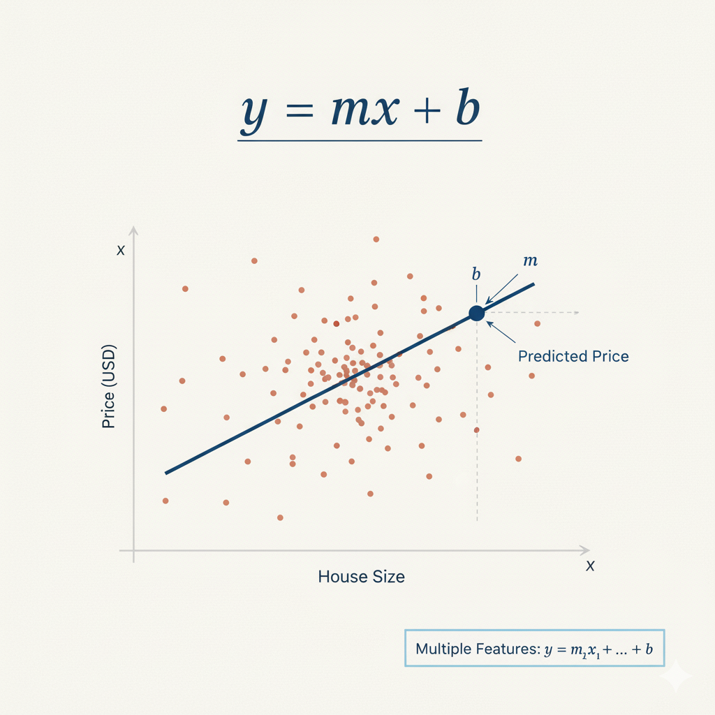 图 1:线性回归公式 y = mx + b,其中 m 是斜率,b 是截距
将以下代码追加到你的 main.py 文件中。这将导入 LinearRegression 类并创建一个模型对象。
from sklearn.linear_model import LinearRegression

## Initialize the Linear Regression model
model = LinearRegression()

## Print the model to confirm it's created
print("\n--- Model Initialized ---")
print(model)
在终端中再次运行你的 main.py 脚本:
python3 main.py
输出现在将包含一行显示 LinearRegression 对象的内容。这确认模型已成功初始化。
--- Model Initialized ---
LinearRegression()
使用 model.fit(X_train, y_train) 拟合模型
在这一步中,我们将训练模型。这个过程通常被称为将模型“拟合”(fitting)到数据上。在拟合过程中,模型会学习特征(X_train)与目标变量(y_train)之间的关系。对于线性回归,这意味着找到每个特征的最佳系数,以最准确地预测目标。
我们将使用模型对象的 fit() 方法,并将训练数据作为参数传递。
将以下代码追加到你的 main.py 文件中。
## Fit (train) the model on the training data
## The fit() method learns the relationship between features (X_train) and target (y_train)
## It calculates optimal coefficients for each feature and the intercept using least squares optimization
model.fit(X_train, y_train)

## After fitting, the model has learned the coefficients and intercept.
## The intercept represents the predicted value when all features are zero
print("\n--- Model Trained ---")
print("Intercept:", model.intercept_)
现在,从终端执行脚本:
python3 main.py
脚本运行后,你将在输出中看到一个新部分,显示线性回归模型的截距。截距是当所有特征值均为零时的预测值。在这里看到数值确认了模型已成功在数据上完成训练。
--- Model Trained ---
Intercept: -37.023277706064185
使用 model.predict(X_test) 在测试数据上进行预测
在最后一步中,我们将使用训练好的模型进行预测。这是构建预测模型的最终目标。我们将使用模型在训练期间未见过的测试数据(X_test)来评估其性能。
我们将使用训练好的模型对象的 predict() 方法,并将测试特征(X_test)作为参数传递。该方法将返回目标变量的预测值数组。
将以下代码追加到你的 main.py 文件中。
## Make predictions on the test data
## The predict() method uses the learned coefficients and intercept to calculate predictions
## Formula: prediction = intercept + (coeff1 * feature1) + (coeff2 * feature2) + ...
predictions = model.predict(X_test)

## Print the first 5 predictions (values are in $100,000 units)
print("\n--- Predictions ---")
print(predictions[:5])
现在,最后一次从终端运行完整脚本:
python3 main.py
输出现在将包含测试集的前五个预测房价。这些值是我们的模型根据 X_test 中的特征认为的房价中位数。你可以从概念上将这些预测值与 y_test 中的实际值进行比较,以衡量模型的准确性。
--- Predictions ---
[0.71912284 1.76401657 2.70965883 2.83892593 2.60465725]
恭喜!你已经成功使用 scikit-learn 构建、训练并使用了一个线性回归模型。
使用 matplotlib.pyplot.scatter() 可视化模型预测结果
在最后一步中,我们将创建一个可视化图表,以更好地了解模型的性能。可视化在机器学习中至关重要,因为它能帮助我们发现从原始数字中可能不明显的模式和关系。
我们将创建一个散点图,比较实际房价(y_test)与我们模型的预测值。这种图被称为“预测值 vs 实际值”散点图。如果我们的模型是完美的,所有点都将位于对角线(45 度线)上,即预测值等于实际值。
我们将使用 matplotlib 创建此可视化图表并将其保存为图像文件。
将以下代码追加到你的 main.py 文件中:
import matplotlib.pyplot as plt

## Create a scatter plot comparing actual vs predicted values
plt.figure(figsize=(10, 6))
plt.scatter(y_test, predictions, alpha=0.5, color='blue', edgecolors='black')

## Add a diagonal line showing perfect predictions (where predicted = actual)
plt.plot([y_test.min(), y_test.max()], [y_test.min(), y_test.max()],
         'r--', linewidth=2, label='Perfect Prediction')

## Add labels and title
plt.xlabel('Actual House Prices ($100,000)')
plt.ylabel('Predicted House Prices ($100,000)')
plt.title('Linear Regression: Actual vs Predicted House Prices')
plt.legend()
plt.grid(True, alpha=0.3)

## Save the plot to a file
plt.savefig('housing_predictions.png', dpi=300, bbox_inches='tight')
plt.close()

print("\n--- Visualization Complete ---")
print("Plot saved to housing_predictions.png")
现在,从终端运行完整脚本:
python3 main.py
你将看到一条确认消息,说明图表已保存。
--- Visualization Complete ---
Plot saved to housing_predictions.png
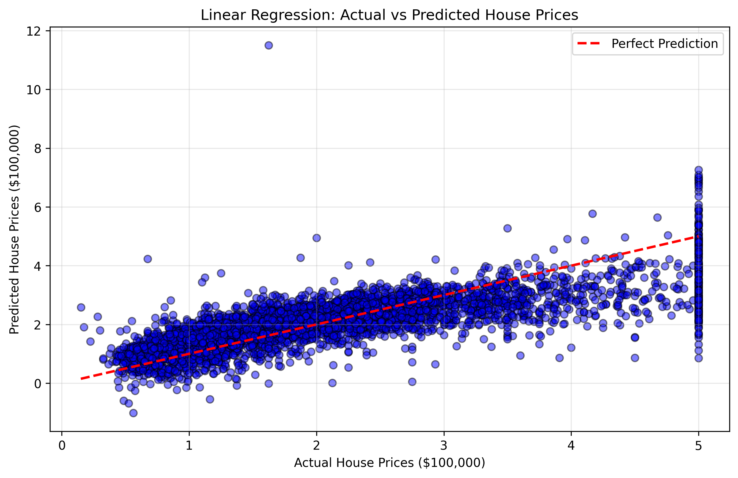 图 2:显示实际房价与预测房价的散点图。越靠近红色对角线的点表示预测越准确。
此可视化图表将帮助你了解:
- 靠近对角线的点:模型准确的良好预测。
- 远离对角线的点:模型产生较大误差的较差预测。
- 整体模式:模型在某些价格范围内是倾向于高估还是低估。
你可以双击文件资源管理器中的 housing_predictions.png 文件来查看你的可视化结果。
恭喜!你已经成功使用 scikit-learn 构建、训练、测试并可视化了一个线性回归模型。
总结
在本实验中,你完成了使用 scikit-learn 构建基础机器学习模型的完整工作流程。
你首先加载了加利福尼亚州住房数据集,并使用 pandas 对其进行了准备。然后,你了解了将数据拆分为训练集和测试集的重要性,并使用 train_test_split 执行了拆分。
随后,你初始化了一个 LinearRegression 模型,使用 fit() 方法在训练数据上对其进行了训练,使用训练好的模型通过 predict() 方法对未见过的测试数据进行了预测,最后可视化了结果以了解模型的性能。
本实验为你打下了坚实的 scikit-learn 基础。在此基础上,你可以探索更高级的主题,例如:
- 模型评估:计算均方误差(MSE)或 R 平方(R-squared)等指标来衡量模型准确性。
- 数据可视化:创建更高级的图表,如残差图、特征重要性图或相关矩阵。
- 特征缩放:标准化或归一化特征以获得更好的性能。
- 正则化:使用岭回归(Ridge)或套索回归(Lasso)来防止过拟合。
- 交叉验证:使用 k 折交叉验证进行更稳健的评估。
- 其他算法:尝试随机森林(Random Forest)、支持向量机(SVM)或神经网络。